Principal Component Analysis
A principal component analysis is a mathematical analysis that identifies and quantifies the directions of variability in the data. For a set of samples, e.g. an experiment, this can be done either by finding the eigenvectors and eigenvalues of the covariance matrix of the samples or the correlation matrix of the samples (the correlation matrix is a 'normalized' version of the covariance matrix: the entries in the covariance matrix look like this ![]() , and those in the correlation matrix like this:
, and those in the correlation matrix like this:
![]() . A covariance maybe any value, but a correlation is always between -1 and 1).
. A covariance maybe any value, but a correlation is always between -1 and 1).
The eigenvectors are orthogonal. The first principal component is the eigenvector with the largest eigenvalue, and specifies the direction with the largest variability in the data. The second principal component is the eigenvector with the second largest eigenvalue, and specifies the direction with the second largest variability. Similarly for the third, etc. The data can be projected onto the space spanned by the eigenvectors. A plot of the data in the space spanned by the first and second principal component will show a simplified version of the data with variability in other directions than the two major directions of variability ignored.
To start the analysis:
Tools | Microarray Analysis (![]() )| Quality Control (
)| Quality Control (![]() ) | Principal Component Analysis (
) | Principal Component Analysis (![]() )
)
Select a number of samples ( (![]() ) or (
) or (![]() )) or an experiment (
)) or an experiment (![]() ) and click Next.
) and click Next.
This will display a dialog as shown in figure 35.37.
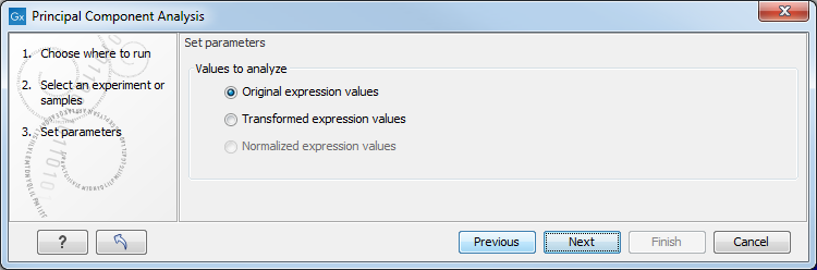
Figure 35.37: Selecting which values the principal component analysis should be based on.
In this dialog, you select the values to be used for the principal component analysis (see Selecting transformed and normalized values for analysis).
Click on Finish to launch the analysis.
Subsections