Map Bisulfite Reads to Reference
Setting up the Map Bisulfite Reads to Reference tool is very similar to the usual read mapping, with a few differences. In particular,
- Some options such as 'Global alignment' are either not available or preset.
- Only a track version of mappings is produced in output.
- The bisulfite mappings have a special 'invisible' property set for them, to inform Call Methylation Levels about the correct type of input.
Please note that, because two versions of the reference sequence (C->T and G->A - converted) have to be indexed and used simultaneously for each read, the RAM requirements for the bisulfite mapper are double than those needed for a regular mapping against a reference sequence of the same size.
To start the read mapping:
Tools | Epigenomics Analysis (![]() ) | Bisulfite Sequencing (
) | Bisulfite Sequencing (![]() )| Map Bisulfite Reads to Reference (
)| Map Bisulfite Reads to Reference (![]() )
)
Selecting reads and directionality
In the first dialog, select the sequences or sequence lists containing the sequencing data (figure 37.15). Please note that reads longer than 100,000 bases are not supported.
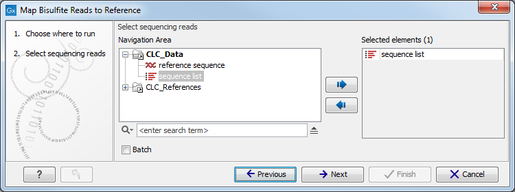
Figure 37.15: Specifying the reads as input. You can also choose to work in batch.
When the sequences are selected, click Next to specify what type of protocol you have used (directional or not).
A directional protocol yields reads from both strands of the original sample-DNA. The first read of a pair (or every read for single-end sequencing) is known to be sequenced either from the original-top (OT) or the original-bottom (OB) strand. The second read of a pair is sequenced from a complementary strand, either ctOT or ctOB. At the time of writing, examples of directional protocols include:
- Illumina TruSeq DNA Methylation Kit (formerly EpiGnome)
- Kits from the NuGen Ovation family of products
- Swift Accel-NGS Methyl-seq DNA Library Kit
- Libraries prepared by the 'Lister' method
In a non-directional protocol, the first read of a pair may come from any of the four strands: OT, OB, ctOT or ctOB. Examples include:
- QIAseq Methyl Library Kit
- Zymo Pico Methyl-Seq Library Kit
- Bioo Scientific (Perkin Elmer) NEXTflex Bisulfite-Seq Kit
- Libraries prepared by the 'Cokus' method
If you are uncertain about the directionality of your protocol, contact the protocol vendor. Note that it is sometimes possible to infer the directionality by looking at the reads: in the absence of methylation, a directional protocol will have few or no Cs in the first read of each pair. We do not recommend however using this approach.
Selecting the reference
When the sequences and directionality are selected, click Next, and you will see the dialog shown in figure 37.16.
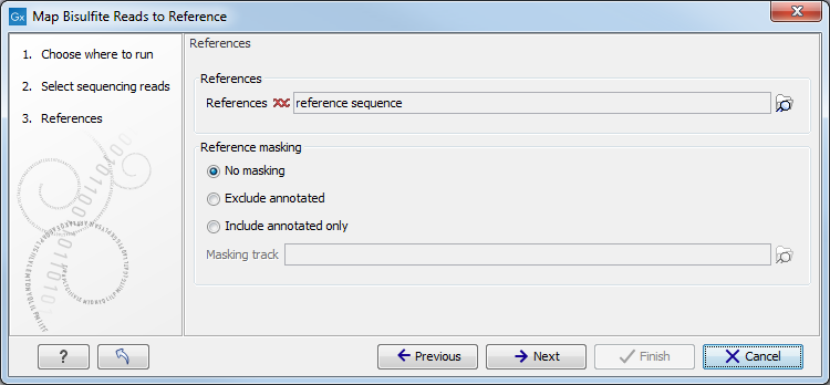
Figure 37.16: Specifying the reference sequences and masking.
Click the Browse and select element (![]() ) button to
select either single sequences, a list of sequences or a sequence
track as reference. Note the following constraints:
) button to
select either single sequences, a list of sequences or a sequence
track as reference. Note the following constraints:
- single reference sequences longer than 2gb (
 bases) are not supported.
- a maximum of 120 input items (sequence lists or sequence elements) can be used as input to a single read mapping run.
Reference masking
The next part of the dialog lets you mask the reference. Masking means that selected regions of the reference are ignored during read mapping. Reads will not be mapped to these regions, but the full reference is still included in the output.
Masking can be useful when reads are expected to originate only from specific regions, for example when working with targeted sequencing data. However, masking should be used with care. If reads originate outside the selected regions, they may be mapped to less suitable locations, which can affect downstream analyses such as variant detection.
Masking large numbers of regions, such as repetitive sequences, is generally not recommended. Repeats are handled automatically during mapping, and masking them may reduce performance and lead to incorrect read placement.
To mask a reference using regions defined in a masking track, choose:
- Include annotated only to map reads only to those regions.
- Exclude annotated to ignore those regions.
If your regions are stored as sequence annotations, they can be converted to a track.
Mapping parameters
Clicking Next leads to the parameters for the read mapping (see figure 37.17).
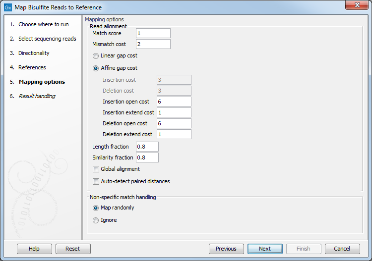
Figure 37.17: Setting parameters for the bisulfite read mapping.
The first parameter allows the mismatch cost to be adjusted:
- Match score The positive score for a match between the read and the reference sequence. It is set by default to 1 but can be adjusted up to 10.
- Mismatch cost The cost of a mismatch between the read and the reference sequence. Ambiguous nucleotides such as "N", "R" or "Y" in read or reference sequences are treated as a mismatches and any column with one of these symbols will therefore be penalized with the mismatch cost.
After setting the mismatch cost you need to choose between linear gap cost and affine gap cost, and depending on the model you chose, you need to set two different sets of parameters that control how gaps in the read mapping are penalized.
- Linear gap cost The cost of a gap is computed directly from the
length of the gap and the insertion or deletion cost. This model
often favors small, fragmented gaps over long contiguous gaps.
If you choose linear gap cost, you must set the insertion cost and the
deletion cost:
- Insertion cost
- The cost of an insertion in the read (a gap in the reference sequence). The cost of an insertion of length
 will be

Insertion cost. - Deletion cost
- The cost of a deletion in the read (gap in the read sequence). The cost of a deletion of length will be
Deletion cost.
- Affine gap cost An extra cost associated with opening a gap is
introduced such that long contiguous gaps are favored over short
gaps.
If you chose affine gap cost, you must also set the cost of opening an
insertion or a deletion:
- Insertion open cost
- The cost of opening an insertion in the read (a gap in the reference sequence).
- Insertion extend cost
- The cost of extending an insertion in the read (a gap in the reference sequence) by one column.
- Deletion open cost
- The cost of a opening a deletion in the read (gap in the read sequence).
- Deletion extend cost
- The cost of extending a deletion in the read (gap in the read sequence) by one column.
Using affine gap cost, an insertion of length
is penalized by
Insertion open cost+ Insertion extend costand a deletion of length
is penalized by
Deletion open cost+ Deletion extend costIn this way long consecutive gaps get a lower cost per column than small fragmented gaps and they are therefore favored.
The score of a match between the read and the reference is usually set to 1. Adjusting the cost parameters above can improve the mapping quality, e.g. when the read error rate is high or the reference is expected to differ significantly from the sequenced organism. For example, if the reads are expected to contain many insertions and/or deletions, it can be a good idea to lower the insertion and deletion costs to allow more of such errors. However, one should also consider the possible drawbacks when adjusting these settings. For example, reducing the insertion and deletion cost increases the risk of mapping reads to the wrong positions in the reference.

Figure 37.18: An alignment of a read where a region of 35bp at the start of the read is unaligned while the remaining 57 nucleotides matches the reference.
Figure 37.18 shows an example using linear
gap cost where the read mapper is unable to map a region in a read
due to insertions in the read and mismatches between the read and
the reference. The aligned region of the read has a total of 57
matching nucleotides which result in an alignment score of 57 which
is optimal when using the default cost for mismatches and insertions/deletions (2 and 3 respectively). If the mapper had aligned the remaining 35bp
of the read as shown in figure 37.19 using
the default scoring scheme, the score would become:
(26+1+3+57)*1 - 5*2 - 8*3 = 53
In this case, the alignment shown in Figure 37.18 is optimal since it has the highest score. However, if either the cost of deletions or mismatches were reduced by one, the score of the alignment shown in figure 37.19 would become 61 and 58, respectively, and thus make it optimal.

Figure 37.19: An alignment of a read containing a region with several mismatches and deletions. By reducing the default cost of either mismatches or deletions the read mapper can make an alignment that spans the full length of the read.
Once the optimal alignment of the read is found, based on the cost parameters described above, a filtering process determines whether this match is good enough for the read to be included in the output. The filtering threshold is determined by two factors:
- Length fraction The minimum percentage of the total alignment
length that must match the reference sequence at the selected
similarity fraction. A fraction of 0.5 means that at least half of
the alignment must match the reference sequence before the read is
included in the mapping (if the similarity fraction is set to
1). Note, that the minimal seed (word) size for read mapping is 15
bp, so reads shorter than this will not be mapped.
- Similarity fraction The minimum percentage identity between the aligned region of the read and the reference sequence. For example, if the identity should be at least 80% for the read to be included in the mapping, set this value to 0.8. Note that the similarity fraction relates to the length fraction, i.e. when the length fraction is set to 50% then at least 50% of the alignment must have at least 80% identity (see figure 37.20).
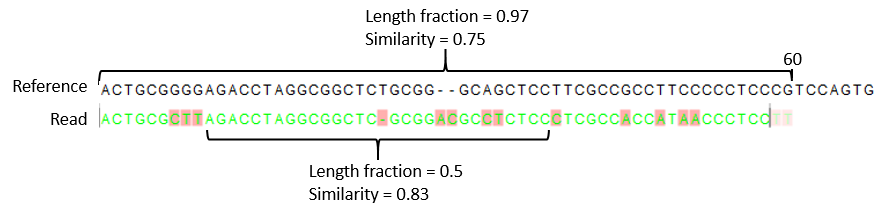
Figure 37.20: A read containing 59 nucleotides where the total alignment length is 60. The part of the alignment that gave rise to the optimal score has length 58 which excludes 2 bases at the left end of the read. The length fraction of the matching region in this example is therefore 58/60 = 0.97. Given a minimum length fraction of 0.5, the similarity fraction of the alignment is computed as the maximum similarity fraction of any part of the alignment which constitute at least 50% of the total alignment. In this example the marked region in the alignment with length 30 (50% of the alignment length) has a similarity fraction of 0.83 which will satisfy the default minimum similarity fraction requirement of 0.8.
Mapping paired reads
- Global alignment By default, mapping is done with local alignment of the reads to the reference. The advantage of performing local
alignment instead of global alignment is that the ends are automatically left unaligned if there are many differences from the reference at the ends. For many sequencing platforms, the quality of the bases drop along the read, and a local alignment approach is desirable. By checking this option, the mapper is forced to look for the highest scoring alignment of the entire read, meaning that the read mapping generated will have no unaligned ends even when the end of the reads align to the wrong places.
- Auto-detect paired distances If the sequence list used as input contains paired reads, this option will automatically be enabled - if it contains single reads, this option will not be applicable.
CLC Genomics Workbench offers as the default choice to automatically calculate the distance between the pairs. If this is selected, the distance is estimated in the following way:
- A sample of 200,000 reads is extracted randomly from the full data set and mapped against the reference using a very wide distance interval.
- The distribution of distances between the paired reads is analyzed using a method that investigates the shape of the distribution and finds the boundaries of the peak.
- The full sample is mapped using this distance interval.
- The history (
 ) of the result records the distance interval used.
The above procedure will be run for each sequence list used as input, assuming that they do not necessarily share the same library preparation and could have different distributions of paired distances. Figure 37.21 shows an example of the distribution of intervals with and without automatic pair distance interval estimation.
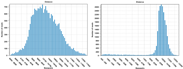
Figure 37.21: To the left: mapping with a narrower distance interval estimated by the workbench. To the right: mapping with a large paired distance interval (note the large right tail of the distribution).
Sometimes the automatic estimation of the distance between the pairs may return a warning "Few reads mapped as pairs so pair distance might not be accurate". This message indicates that the paired distance was chosen to spans all uniquely mapped reads. If in doubt, you may want to disable the option to automatically estimate paired distances and instead manually specify minimum and maximum distances between pairs on the input sequence list.
If the automatic detection of paired distances is not checked, the mapper will use the information about minimum and maximum distance recorded on the input sequence lists.
When a paired distance interval is set, the following approach is used for determining the placement of read pairs:
- First, all the optimal placements for the two individual reads
are found.
- Then, the allowed placements according to the paired distance interval are found.
- If both reads can be placed independently but no pairs
satisfies the paired criteria, the reads are treated as
independent and marked as a broken pair.
- If only one pair of placements satisfy the criteria, the reads
are placed accordingly and marked as uniquely placed even if either
read may have multiple optimal placements.
- If several placements satisfy the paired criteria, the pair
is treated as a non-specific match (see Non-specific matches for more information.)
- If one read is uniquely mapped but the other read has several placements that are valid given the distance interval, the mapper chooses the location that is closest to the first read.
Non-specific matches
At the bottom of the dialog, you can specify how Non-specific matches should be treated. The concept of Non-specific matches refers to a situation where a read aligns at more than one position with an equally good score. In this case you have two options:
- Random. This will place the read in one of the positions randomly.
- Ignore. This will not include the read in the final mapping.
Note that a read is only considered non-specific when the read matches equally well at several alignment positions. If there are e.g. two possible alignment positions and one of them is a perfect match and the other involves a mismatch, the read is placed at the position with the perfect match and it is not marked as a non-specific match.
For paired data, reads are only considered non-specific matches if the entire pair could be mapped elsewhere with equal scores for both reads, or if the pair is broken in which case a read can be categorized as non-specific in the same way as single reads (see Mapping paired reads).
When looking at the mapping, the default color for non-specific matches is yellow.
Gap placement
In the case of insertions or deletions in homopolymeric or repetitive regions, the precise placement of the insertion or deletion cannot be determined from the data. An example is shown in figure 37.22.
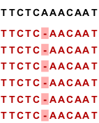
Figure 37.22: Three A's in the reference (top) have been replaced by two A's in the reads (shown in red). The gap is placed towards the 5' end, but could have been placed towards the 3' end with an equally good mapping score for the read.
In this example, three A's in the reference (top) have been replaced by two A's in the reads (shown in red). The gap is placed towards the 5' end (left side), but could have been placed towards the 3' end with an equally good mapping score for the read as shown in figure 37.23.
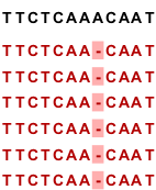
Figure 37.23: Three A's in the reference (top) have been replaced by two A's in the reads (shown in red). The gap is placed towards the 3' end, but could have been placed towards the 5' end with an equally good mapping score for the read.
Since either way of placing the gap is arbitrary, the goal of the mapper is to place the gaps consistently at the same side for all reads.
Bisulfite read mapping result handling
()Click Next lets you choose how the output of the mapping should be reported. There are two independent output options available that can be (de-)activated in both cases:
- Create report. This will generate a summary report as described in Summary mapping report.
- Collect unmapped reads. This will collect all the reads that could not be mapped to the reference into a sequence list (there will be one list of unmapped reads per sample, and for paired reads, there will be one list for intact pairs and one for single reads where the mate could be mapped).
The main output is a reads track. A reads track is very "lean" (i.e. with respect to memory requirements) since it only contains the reads themselves. Additional information about the reference, consensus sequence or annotations can be added and viewed alongside in the context of a Track List later (by adding, for example, a reference and/or annotation track, respectively). This kind of output is useful when working with tracks in general and especially for resequencing purposes this is recommended.
Note that the tool will output an empty read mapping and report when nothing mapped, and empty unmapped reads if everything mapped.
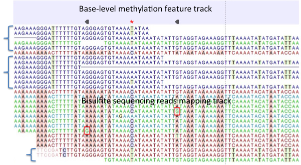
Figure 37.24: A typical directional shotgun BS-seq mapping, together with the base-level methylation calling feature track on top.
Figure 37.24 illustrates the view of a typical directional shotgun BS-seq mapping. As with any read mapping view, the color of the reads follows the usual CLC convention, that is green/red for forward/reverse reads, and dark/pale blue for paired reads. Independent of this orientation property, each read or read pair has an 'invisible' property indicating if it came from the original top (OT), or original bottom (OB) strand. However, if the BS-sequencing protocol is truly 100%-directional, the orientation in the mapping and the OT/OB origin of reads/read pairs will be concordant.
In this figure, blocks of reads from the original top strand are marked with squiggly brackets on the left, while the rest are from the original bottom strand. In a mapping, they can be distinguished by a pattern of highlighted mismatches to reference. OT reads will have mismatches predominantly on 'T', due to C->T conversion; OB reads will have a pattern of mismatches on 'A' symbols, corresponding to G->A conversion as can be seen on a reverse-complementary strand. When methyl-C occurs in a sample, there will be a match in the reads, instead of an expected mismatch.
In this figure, there were two positions where such events occurred, both on the original bottom strand, and both supported by a single read only. 'G' symbols in those reads are shown in red boxes. The reverse direction of an arrowhead on a base-level methylation track also reflects the OB-position of a methylation event.
Note also that it appears that there may be a G/T heterozygous SNP (C/A in the OB strand) in the second position. While such occurrences may lead to underestimation of true methylation levels of cytosine alleles in heterozygous SNPs, our current tool does not attempt to compensate for such eventualities.
To understand and interpret BS-sequencing and mapping better, it may be helpful to examine the position (marked with a red asterisk) in between the two detected methylation events. There appears to be an additional A/C heterozygous SNP with C's in reads from OT strand fully converted to T's, i.e., showing no evidence of methylation at that heterozygous position.