Principal component analysis plot (2D)
The default view is a two-dimensional principal component plot as shown in figure 34.69.
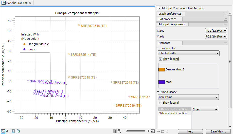
Figure 34.69: A principal component plot.
The plot shows the projection of the samples onto the two-dimensional space spanned by the first and second principal components of the covariance matrix.
The view settings can be adjusted using the Side Panel. Under Graph preferences, you can adjust the general properties of the plot.
- Lock axes This will always show the axes even though the plot is zoomed to a detailed level.
- Frame Shows a frame around the graph.
- Tick type Determines whether tick lines should be shown outside or inside the frame.
- Tick lines at Choosing Major ticks will show a grid behind the graph.
- Horizontal axis range Sets the range of the horizontal axis (x axis). Enter a value in Min and Max, and press Enter. This will update the view. If you wait a few seconds without pressing Enter, the view will also be updated.
- Vertical axis range Sets the range of the vertical axis (y axis). Enter a value in Min and Max, and press Enter. This will update the view. If you wait a few seconds without pressing Enter, the view will also be updated.
- y = 0 axis Draws a line where y = 0 with options for adjusting the line appearance.
Below the general preferences, you find the Dot properties:
- Drop down menu In this you select the expression tracks to which following choices apply.
- Dot type Allows you to choose between different dot types.
- Dot color Click the color box to select a color.
- Show name This will show a label with the name of the sample next to the dot.
Note that the Dot properties may be overridden when the Metadata options are used to control the visual appearance (see below).
The Principal Components group determines which two principal components are used in the 2D plot. By default, the first principal component is shown for the X axis and the second principal component is shown for the Y axis. The value after the principal component identifier (for example "PC1 (72.5 %)") displays the amount of variance explained by this particular principal component.
The Metadata group allows metadata associated with the Expression tracks to be visualized in a number of ways:
- Symbol color Colors are assigned based on a categorical factor in the metadata table.
- Symbol shape Shape is assigned based on a categorical factor in the metadata table.
- Label text Dots are labeled according to the values in a given metadata column.
- Legend font settings contains options to adjust the display of labels.
The graph and axes titles can be edited simply by clicking them with the mouse.