Peak refinement
Clicking Next will display the dialog shown in figure 29.2.
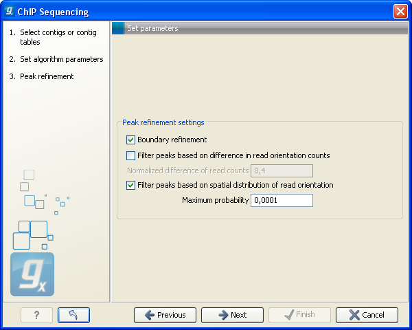
Figure 29.2: Peak refinement settings.
This dialog presents the parameters and options that can be used to refine the set of candidate peaks discovered when scanning the read mapping. All three refinement options again utilize the fact that coverage around a true DNA-protein binding site is expected to exhibit a signature distribution where forward reads are found upstream of the binding site and reverse reads are found downstream of the binding site. Peak refinement can be performed both with- and without a control sample but the algorithm only uses information contained in the reads from the ChIP-samples, not the control samples.
If the Boundary refinement option is checked, the algorithm will estimate the position of the DNA-protein binding interaction and place the resulting annotations on this region, rather than on the region where a peak in coverage is found. A center of sequencing intensity is defined for all forward reads as the median value of the center points of all forward reads and likewise for all reverse reads. The "refined peak" is thus defined as the region between these two points.
One of the advantages of including this boundary refinement is that shorter regions can be given as input to subsequent pattern discovery analysis.
By checking the Filter peaks based on difference in read orientation counts the algorithm will calculate the normalized difference in the number of forward and reverse reads within a peak as
The desired maximum value of this parameter can be set in the Normalized difference of read counts field and any candidate peak with a value above this will then be dismissed. Setting a low value will ensure that peaks are only called if there is a well balanced number of forward and reverse reads.
As an example if you have 15 forward reads and 5 reverse reads, you will end up with a value of 0.5. With the default limit set to 0.4, a peak like that would be excluded.
By checking the Filter peaks based on spatial distribution of read orientation the algorithm will evaluate how clearly separated the location of forward and reverse reads are within a peak. This is done via the Wilcoxon rank-sum test (see http://en.wikipedia.org/wiki/Mann-Whitney-Wilcoxon_test). The null hypothesis here is that the positions of forward and reverse reads within a peak are drawn from the same distribution i.e. that their locations are not significantly different and the alternative hypothesis is that the forward reads have a sum of ranked positions that is shifted to lower positions than the reverse reads. Peaks will be dismissed if the probability of the null hypothesis exceeds the value set in the Maximum probability field.
Setting a low Maximum probability will ensure that peaks are only called if there is a clear signature distribution where forward reads are found upstream of reverse reads within the peak.
A general comment about peak filtering is that the relevant statistics are all reported in the peak table that the algorithm outputs. If it is desirable to explore a large set of candidate peaks it is recommended to use no or relatively loose filtering criteria and then use the advanced table filtering options to explore the effect of the different parameters (see Working with tables). It may be desirable to omit the addition of annotations in this exploratory analysis and rely on the information in the table instead. Once a desired set of parameters is found, the algorithm can be rerun using these as filtering criteria to add annotations to the reference sequence and to produce a final list of peaks.