Peak finding and false discovery rates
Clicking Next will display the dialog shown in figure 29.1.
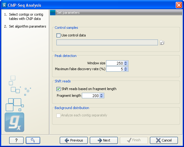
Figure 29.1: Peak finding and false discovery rates.
If the option to include control samples is included, the user must select the appropriate sample to use as control data. If the mapping is based on several reference sequences, the Workbench will automatically match the ChIP-samples and controls based on the length of the reference sequences.
The peak finding algorithm includes the following steps:
- Calculate the null distribution of background sequencing signal
- Scan the mappings to identify candidate peaks with a higher read count than expected from the null distribution
- Merge overlapping candidate peaks
- Refine the set of candidate peaks based on the count and the spatial distribution of reads of forward and reverse orientation within the peaks
The estimation of the null distribution of coverage and the calculation of the false discovery rates are based on the Window size and Maximum false discovery rate (%) parameters. The Window size specifies the width of the window that is used to count reads both when the null distribution is estimated and for the subsequent scanning for candidate peaks.
The Maximum false discovery rate specifies the maximum proportion of false positive peaks that you are willing to accept among your called peaks. A value of 10 % means that you are willing to accept that 10 % of the peaks called are expected to be false discoveries.
To estimate the false discovery rate (FDR) we use the method of [Ji et al., 2008] (see also Supplementary materials of the paper).
In the case where only a ChIP-sample is used, a negative binomial distribution is fitted to the counts from low coverage regions. This distribution is used as a null distribution to obtain the numbers of windows with a particular count of reads that you would expect in the absence of significant binding. By comparing the number of windows with a specific count you expect to see under the null distribution and the number you actually see in your data, you can calculate a false discovery rate for a given read count for a given window size as: 'fraction of windows with read count expected under the null distribution'/'fraction of windows with read count observed'.
In the case where both a ChIP- and a control sample are used, a sampling ratio between the samples is first estimated, using only windows in which the total numbers of reads (that is, the sum of those in the sample and those in the control) is small. The sampling ratio is estimated as the ratio of the cumulated sample read counts (
![]() ) to cumulated control read counts (
) to cumulated control read counts (
![]() ) in these windows. The sampling ratio is used to estimate the proportion of the reads that are expected to be ChIP-sample reads under the null distribution, as
) in these windows. The sampling ratio is used to estimate the proportion of the reads that are expected to be ChIP-sample reads under the null distribution, as
![]() . For a given total read count, n, of a window, the numbers of reads expected in the ChIP-sample under the null distribution can then be estimated from the binomial distribution with parameters n and
. For a given total read count, n, of a window, the numbers of reads expected in the ChIP-sample under the null distribution can then be estimated from the binomial distribution with parameters n and ![]() . By comparing the expected and observed numbers, a false discovery rate can then be calculated. Note, that when a control sample is used different null-distributions are estimated for different total read counts, n.
. By comparing the expected and observed numbers, a false discovery rate can then be calculated. Note, that when a control sample is used different null-distributions are estimated for different total read counts, n.
In both cases, the user can specify whether the null distribution should be estimated separately for each reference sequence by checking the option Analyze each reference separately.
Because the ChIP-seq experimental protocol selects for sequencing input fragments that are centered around a DNA-protein binding site it is expected that true peaks will exhibit a signature distribution where forward reads are found upstream of the binding site and reverse reads are found downstream of the binding site leading to reduced coverage at the exact binding site. For this reason, the algorithm allows you to shift forward reads towards the 3' end and reverse reads towards the 5' end in order to generate a more marked peak prior to the peak detection step. This is done by checking the Shift reads based on fragment length box. To shift the reads you also need to input the expected length of the sequencing input fragments by setting the Fragment length parameter, this is the size of the fragment isolated from gel (L in the illustration below).
The illustration below shows a peak where the forward reads are in one window and the reverse reads fall in another window (window 1 and 3).
--------------------------------------------------------- reference
        ----------------------|------------------         (actual sequenced fragment length = L bp)
        ---->                                             reads
         ---->                                            reads
                                             <---         reads
                                           <---           reads.
|--------------------|--------------------|-------------  window size W
         1                      2                  3
If the reads are not shifted, the algorithm will count 2 reads in window 1 and 3. But if the forward reads are shifted 0.5XL to the right and reverse reads are shifted 0.5xL to left, the algorithm will find 4 reads in window 2 as shown below:
--------------------------------------------------------- reference
        ----------------------|------------------         (actual sequenced fragment length = L basepairs)
                              ---->                         reads
                               ---->                        reads
                           <---                             reads
                          <---                              reads
|--------------------|--------------------|-------------  window size W
         1                      2                  3
So shifting reads will increase the signal to noise ratio.
The following peak refinement step, the reporting of the peak and the visualization will use the original position of the reads, so the shifting is only a virtual shift performed as part of the peak detection.