Type a Known Species
The Type a Known Species workflow is designed for typing of samples representing a single known species. It identifies the associated MLST, determines variants found when mapping the sample data against the specified reference, and finds occurring resistance genes if they match genes within the specified resistance database.
Preliminary steps to run the Type a Known Species workflow
Before starting the workflow,
- Download microbial genomes using either Download Custom Microbial Reference Database, the prokaryotic databases from Download Curated Microbial Reference Database, or using Download Pathogen Reference Database.
- Download the MLST schemes using the Download MLST Scheme tool (see Download MLST Scheme).
- Download the database for the Find Resistance with Nucleotide Database tool using the Download Resistance Database tool (see the Download Resistance Database section).
- Create a New Result Metadata table using the Create Result Metadata Table tool (see the Create Result Metadata Table section).
How to run the Type a Known Species workflow
To run the workflow, go to:
Workflows | Template Workflows (![]() ) | Microbial Workflows (
) | Microbial Workflows (![]() ) | Typing and Epidemiology (
) | Typing and Epidemiology (![]() ) | Type a Known Species (
) | Type a Known Species (![]() )
)
- Specify the sample(s) or folder(s) of samples you would like to type and click Next. Remember that if you select several items, they will be run as batch units.
- Specify the Result Metadata Table you want to add your results to and click Next.
- Define batch units. For details, see Running part of a workflow multiple times.
- Check that batching is as intended.
- If your reads contain adapters, add an appropriate Trim adapter list. Click Next.
- Choose the Reference for Map Reads to Reference (figure 2.27). Click Next.
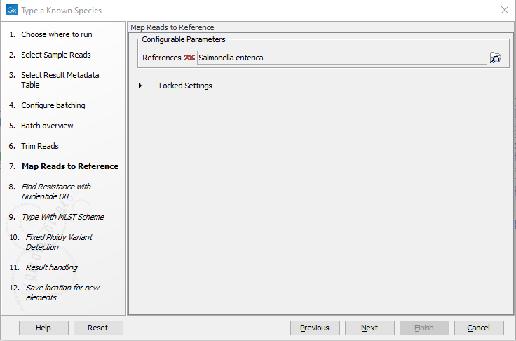
Figure 2.27: Specify the reference for the Map Reads to Reference tool. - Specify the Resistance Database (figure 2.28) and set the parameters for the Find Resistance with Nucleotide Database tool.
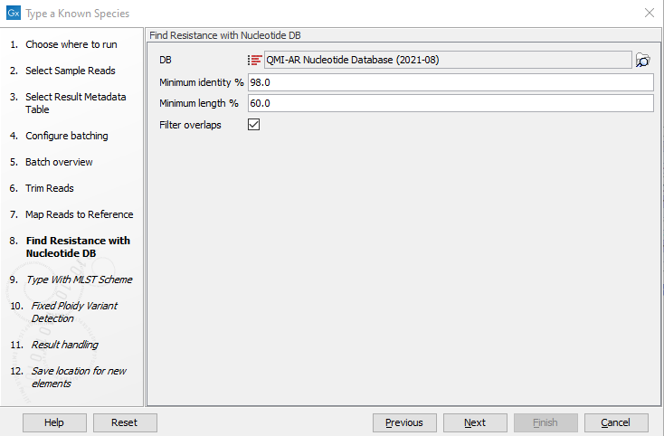
Figure 2.28: Specify the resistance database to be used for the Find Resistance with Nucleotide Database tool.The parameters that can be set are:
- Minimum identity %. The threshold for the minimum percentage of nucleotides that are identical between the best matching resistance gene in the database and the corresponding sequence in the genome.
- Minimum length %. The percentage of the resistance gene length that a sequence must overlap to count as a hit for that gene.
- Filter overlaps. Extra filtering of results per contig, where one hit is contained by the other with a preference for the hit with the higher number of aligned nucleotides (length * identity).
- Specify the MLST Scheme and set the parameters for the Type with MLST Scheme tool (figure 2.29).
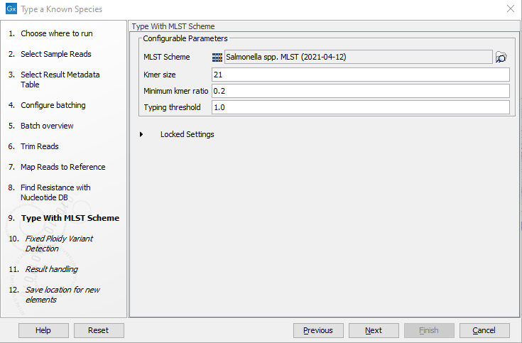
Figure 2.29: Specify the parameters for MLST typing.The parameters that can be set are:
- Kmer size. Determines the number of nucleotides in the kmer - raising this setting might increase specificity at the cost of some sensitivity.
- Minimum kmer ratio. The minimum kmer ratio of the least occurring kmer and the average kmer hit count. If an allele scores higher than this threshold it is classified as a high-confidence call.
- Typing threshold. The typing threshold determines how many of the kmers in a sequences type need be identified before a typing is considered conclusive. The default setting of 1.0 means that all kmers in all alleles must be matched. Lowering the setting to 0.99 would mean that on avergae 99% of all kmers in all the alleles of a given sequence type must be detected before the sequence type is considered conclusive.
Click Next.
- Specify the parameters for the Fixed Ploidy Variant Detection tool (figure 2.30) before clicking Next. For detailed information about all the filters, see Fixed Ploidy Variant Detection and Variant Detection - filters.
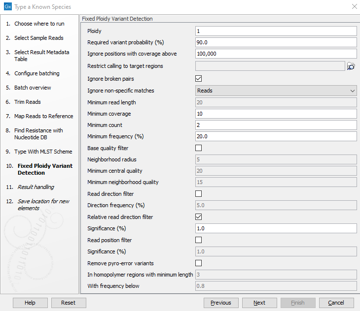
Figure 2.30: Specify the parameters to be used for the Fixed Ploidy Variant Detection tool. - In the "Create Sample Report" step various summary items have been set. These are guidelines to help evaluate the quality of the results (see Create Sample Report).
- In the Result handling window, pressing the button Preview All Parameters allows you to preview - but not change - all parameters. Choose to save the results (we recommend to create a new folder for it) and click Finish.
The output will be saved in the location you chose, and eligible results will also be added automatically to the Metadata Result table.
The batch-specific outputs provided by this workflow are:
- Sample report. The sample report is curated to contain the most important information for analysis interpretation. All full reports are linked throughout the Sample report or can be found in the QC & Reports folder. The Sample report icon will be colored based on whether Summary item thresholds were met. See the "Quality control" section in the sample report for specifics.
- Resistance Results. Folder containing results from de novo assembly and resistance calling.
- Assembled contigs list. Contig list from the De novo assembly tool.
- Resistance table. The result table from the Find Resistance with Nucleotide Database tool, reporting the found resistance.
- Typing Results. Folder containing results from typing and variant calling.
- Sequence lists. List(s) of the sequences that were successfully trimmed and mapped to the best reference.
- Read mapping. Mapping of the reads to the specified reference.
- Typing result. Output from the Type with MLST Scheme tool, including information on kmer fractions, kmer hit counts, and alleles identified and called.
- Variant track. Output from the Fixed Ploidy Variant Detection tool. Note: Multiple variant track files from monoploid data that are based on the same reference genome can be exported to a single VCF file using the Multi-VCF exporter.
- QC & Reports. Folder containing the individual reports generated during the analysis.
- All reports from the sample report are found here in their full length.
The combined outputs provided by this workflow are:
- Combined report. Combined report of all sample reports. The combined report contains all quality control information and analysis results. The combined report icon will be colored based on whether Summary item thresholds were met in each sample. See the "Quality control" section in the combined report for specifics.
- Results Metadata Table. A table containing summary information of results for each sample analyzed and a quick way to find the associated files.
Through the Result Metadata Table, it is possible to filter among sample metadata and analysis results. By clicking Find Associated Data (![]() ) and optionally performing additional filtering, it is possible to perform additional analyses on a selected subset directly from this Table, such as:
) and optionally performing additional filtering, it is possible to perform additional analyses on a selected subset directly from this Table, such as:
- Generation of SNP trees based on the same reference used for read mapping and variant detection (Create SNP Tree).
- Generation of K-mer Trees for identification of the closest common reference across samples (Create K-mer Tree).
- Run validated workflows (workflows that are associated with a Result Metadata Table and saved in your Navigation Area).