Detect Amplicon Sequence Variants output
Click Next to select the output (figure 5.14).

Figure 5.14: Detect Amplicon Sequence Variants output options
In addition to an ASV abundance table, the following outputs are available:
- Click Create ASV sequence list to generate a sequence list with the detected amplicon sequence variants.
- Click Create report to generate a summary report.
The ASV report

Figure 5.15: First sections of the Detect Amplicon Sequence Variants report
- Summary (figure 5.15)
- Sample name The name of the sample.
- Input reads The number of input reads.
- Unique sequences The number of unique sequences detected in the input reads. Read pairs are counted as one.
- Amplicon sequences variants The number of amplicon sequences variant detected in the input reads. Read pairs are counted as one.
- Reads in amplicon sequence variants The number of reads grouped into ASVs.
- Read filtering
- Input reads The number of input reads.
- Filtered on length The number of reads that were removed because they were shorter than the defined length threshold.
- Filtered on ambiguity The number of reads that were removed because they contained ambiguous bases.
- Filtered on expected errors The number of reads that were removed because they exceeded the Maximum expected errors threshold.
- Filtered total The total number of filtered reads.
- Filtered (%) The percentage of reads filtered.
- Reads after filtering The number of reads left after filtering.
- Distribution of expected errors
- Read lengths Plot of read lengths before and after length trimming and filtering.
- Unique sequences
- Merging of unique read pairs
- Number of unique pairs The number of read pairs.
- Unique pair with insufficient overlap The number of pairs that had insufficient overlap and were discarded.
- Merged unique pairs The number of read pairs that were successfully merged.
- Error model estimation
- R1 Error model computed based on forward reads.
- R2 Error model computed based on reversed reads.
The ASV abundance table
The ASV abundance table contains the detected amplicon sequence variants (ASVs) and the abundance of each ASV. The Detect Amplicon Sequence Variants tool produces one ASV abundance table per sample. To go beyond single sample ASVs, you can combine tables and enrich them with metadata using the following tools:
- Merge Abundance Tables Creates a merged, multi-sample ASV abundance table that allows you to compare abundances across samples, see Merge Abundance Tables.
- Add Metadata to Abundance Table Adds sample metadata to your table. This allows you to aggregate samples based on attributes. This is useful for instance when analyzing replicates from the same sample origin. See Add Metadata to Abundance Table for information on how to add metadata.
- Assign Taxonomies to Sequences in Abundance Table Assigns taxonomy annotations to the ASVs. You can aggregate ASVs by taxonomy level, (see Assign Taxonomies to Sequences in Abundance Tables).
In the following, we focus on the single sample ASV abundance table, but include a few hints about additional features and options that could be of use for merged ASV abundance tables, ASV abundance tables with sample metadata, and ASV abundance tables with assigned taxonomies.
There are a number of ways to visualize the ASV abundance table:
- Table view (
 ) (figure 5.16)
The table displays the following columns, some of which are of use mostly for merged, multi-sample ASV tables:
- ID The ID of the ASV.
- Name The name of the ASV. The name is generated as an MD5 hash ID, why identical ASVs will have the same name across ASV tables.
- Combined Abundance The total number of reads belonging to the ASV across samples.
- Min Minimum abundance across all samples
- Max Maximum abundance across all samples
- Mean Mean abundance of all samples
- Median Median abundance of all samples
- Std Standard deviation of all samples
- Abundance for each sample The number of reads belonging to the ASV in a specific sample.
- Sequence The sequence of the detected ASV.
In the Data section of the Side panel, switch between Raw and Relative abundance. Relative abundance is computed as the ratio between the number of reads belonging to an ASV and the total number of reads in the sample.
For merged ASV abundance tables with sample metadata, use the setting Aggregate sample to aggregate samples based on metadata attributes, e.g. replicates from the same sample origin.
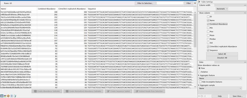
Figure 5.16: The ASV abundance table for a single sampleBelow the table, the following actions are available:
- Create Abundance Subtable will create a table containing only the selected rows.
- Create Sequence Sublist will create a sequence list containing only the selected rows.
For merged ASV abundance tables, an additional action is available:
- Create Normalized Abundance Subtable will create a table with all rows normalized on the values of a single selected row. The row used for normalization will disappear from the new abundance table. The normalization scales the abundance table linearly. The scaling factor is calculated by determining the average abundance across all samples and for each sample scale it to the average for the reference. Note that to be enabled, the selected row must have abundance values for all samples. If you have empty values for some samples for the ASVs you wish to use as control, you will need to generate a new abundance table where those samples are not included. If the abundance table is obtained from merging single-sample abundance tables, then the merge should be redone excluding the samples with zero control read counts.
- Stacked Visualization view (
 )
)
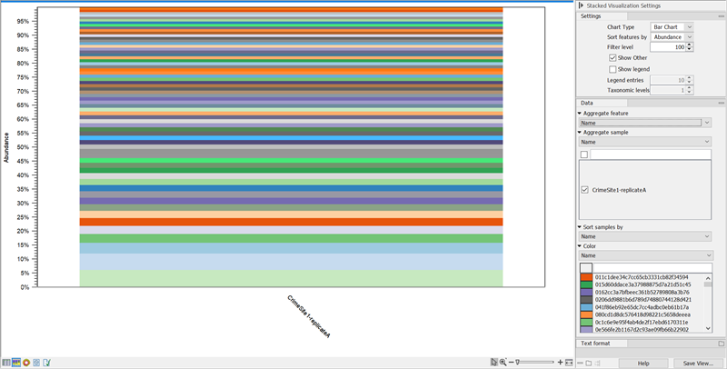
Figure 5.17: The ASV abundance table Stacked Bar Chart with ASVs aggregated on Name shows the relative abundance of ASVs.Adjust the Side panel setting Aggregate feature to Name (figure 5.17) for a visual representation of the relative abundance of ASVs in your sample. Hover over a color to see the name and count of the corresponding ASV.
Use Filter level to adjust the number of features shown in the plot. Setting the value to 10 gives you the 10 most abundant ASVs with remaining ASVs grouped as "Other".
For merged ASV abundance tables, additional Side panel settings may be of use:
- With Chart type you can switch between Bar Chart (figure 5.19) and Area Chart (figure 5.18).
- When sample metadata is applied, use Aggregate sample to aggregate based on metadata attributes e.g. replicates from the same sample origin.
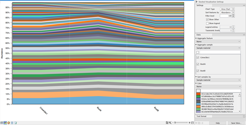
Figure 5.18: Stacked Area Chart of a merged ASV abundance table Area chart, ASVs aggregated on Name, samples aggregated on Sample material. This shows the ASV abundance at 3 different sample sites for a total of 6 samples.For ASV Abundance tables with assigned taxonomies, you can aggregate ASVs by taxonomy level (figure 5.19).
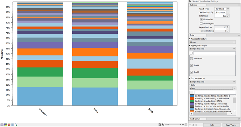
Figure 5.19: Stacked Bar Chart of a merged ASV abundance tables with assigned taxonomies aggregated on Genus level. - Sunburst view (
 )
)
The Sunburst view is only available for ASV abundance tables with assigned taxonomies.
The plot is zoomable. Use Side panel settings to select how many taxonomy levels to display, and how these should be colored. Lower taxonomy levels will inherit the color from higher levels with different shades. Hover over the plot to view a legend with taxonomy and relative abundances for the highlighted section (figure 5.20).
Click on a lower level field to render that field the center of the plot and display lower level counts in a radial view. Click on the center field to render the level above the current view the center of the view.
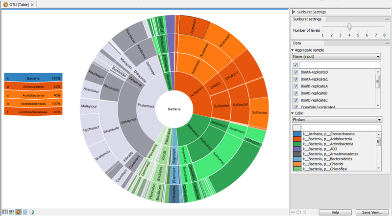
Figure 5.20: Sunburst view of the microbial community showing all taxa belonging to the kingdom bacteria.
