Create SNP Tree
The Create SNP Tree tool is inspired by [Kaas et al., 2014].
To generate a SNP tree, first map reads from the individual samples to a common reference and call variants. The corresponding tools are described at:
- Map Reads To Reference: https://resources.qiagenbioinformatics.com/manuals/clcgenomicsworkbench/current/index.php?manual=Mapping_parameters.html
- Variant detection: https://resources.qiagenbioinformatics.com/manuals/clcgenomicsworkbench/current/index.php?manual=Variant_detection.html
To create a SNP tree, go to:
Tools | Microbial Genomics Module (![]() ) | Typing and Epidemiology (
) | Typing and Epidemiology (![]() ) | Create SNP Tree (
) | Create SNP Tree (![]() )
)
In the first dialog, select reads tracks or read mappings (figure 9.1).
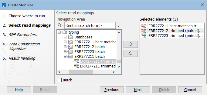
Figure 9.1: Select read mappings to be included in the SNP tree analysis.
Next, select Variant parameters. These determine which SNPs (single-nucleotide polymorphisms) and MNVs (multi-nucleotide variants) to consider for building the SNP tree:
- Variant tracks. Select variant tracks that correspond to the previously selected reads tracks or read mappings (figure 9.2). The variant tracks determine which positions to potentially include in the SNP tree.
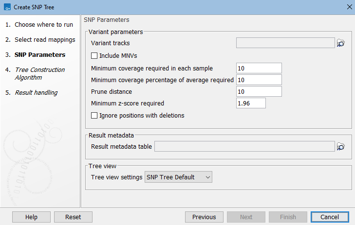
Figure 9.2: Select variant tracks and specify relevant parameters before generation of a SNP tree. - Include MNVs. Check this option to include MNVs along with SNPs when building the SNP tree.
- Minimum coverage required in each sample. Positions are filtered if at least one sample has coverage below the specified threshold.
- Minimum coverage percentage of average required. Positions are filtered if the coverage of at least one sample falls below the specified percentage of the average coverage of that sample.
- Prune distance. Minimum number of nucleotides between unfiltered positions. If a position is within this distance of a previously used position it will be filtered.
- Minimum z-score required. Defining
 as the number of the most prevalent nucleotide at a position and
  as the coverage subtracting
  , the z-score is calculated as
 . If the calculated z-score for a given position is less than the specified minimum value the position is filtered.
The initial list of SNP positions is reduced based on the above filters. Of the remaining, only variants with relative frequency above 50% (haploid organisms) will be considered. SNP positions that overlap a deletion in any sample are not considered, because such SNPs are often false positives caused by undetected deletions in repeat regions. Information about reference and alleles is deduced from the read mappings.
Optionally, select the Result metadata table with metadata relevant for your samples. This will allow you to decorate the resulting SNP tree with metadata information, see SNP tree.
In the next dialog, select the tree construction algorithm (figure 9.3).
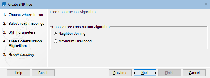
Figure 9.3: Choose the tree construction algorithm.
- Neighbor Joining. Creates a tree with a fast method. In the absence of homoplastic SNPs (a SNP that is acquired independently on different branches of the tree), or positions where three or more nucleotides are present, then the distances in the tree have the following property: If you move from one sample to another in the tree, the sum of the lengths of the branches traversed equals the number of SNP differences between those samples.
- Maximum Likelihood. Calculates the most likely phylogenetic tree under the given evolutionary model. Branch lengths are the number of expected substitutions between samples. For closely related samples these match the number of SNP differences between the samples, as for Neighbor Joining. For more distantly related samples these are expected to exceed the number of SNP differences, and will tend to be systematically too large. This is because distantly related samples are expected to have some positions where multiple substitutions have occurred, and using only SNP positions to build the tree will tend to make samples appear more distantly related than if all positions were used.
In rare cases, a SNP position may be determined to be highly unlikely when constructing a Maximum Likelihood tree. When this happens, the position is removed from the SNP alignment and the tree construction is rerun. The number of SNPs removed this way can be seen in the Post-alignment filtering section of the SNP tree report.
If you selected Maximum Likelihood, the next dialog covers parameters for this algorithm (see figure 9.4). The parameters are described here: https://resources.qiagenbioinformatics.com/manuals/clcgenomicsworkbench/current/index.php?manual=Maximum_Likelihood_Phylogeny.html.
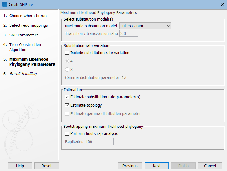
Figure 9.4: Set parameters for maximum likeihood estimation.
In the Result handling dialog, specify the output (figure 9.5).
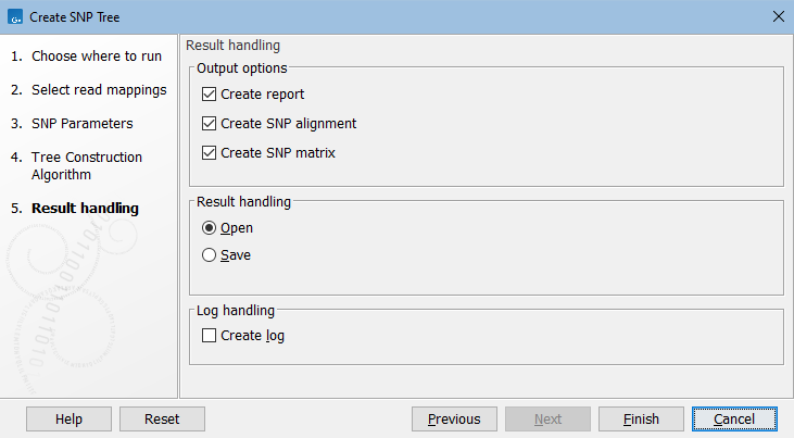
Figure 9.5: Create SNP Tree output options.
In addition to the SNP tree, the following are available:
- Create report. A SNP report with summary of input and results.
- Create SNP alignment. Outputs the alignment that is produced as a first step in the algorithm. The alignment consists of columns of concatenated SNPs and columns of constant A, T, C, and G.
At least 100 constant columns are added to ensure that the equilibrium frequencies of nucleotides more closely resemble those in the reference genome. Additional columns are added until the two most distant sequences in the alignment are 80% identical or until the alignment is the size of the reference genome. This partially mitigates the overestimation of branch lengths when using the Maximum Likelihood tree construction algorithm on SNP positions.
The alignment can be used as input for the Model Testing tool that serves to identify which evolutionary model suits the data best. Based on this, you may want to rerun the Create SNP Tree tool with adjusted settings. The Model Testing tool is described at https://resources.qiagenbioinformatics.com/manuals/clcgenomicsworkbench/current/index.php?manual=Model_Testing.html.
- Create SNP matrix. A matrix containing the number of SNP differences between all pairs of samples.
Subsections
