Compare variants in DNA and RNA
Integrated analysis of genomic and transcriptomic sequencing data is a powerful tool that can help increase our current understanding of human genomic variants. The Compare variants in DNA and RNA ready-to-use workflow identifies variants in DNA and RNA and studies the relationship between the identified genomic and transcriptomic variants.
To run the ready-to-use workflow:
Toolbox | Ready-to-Use Workflows | Whole Transcriptome Sequencing (![]() ) | Compare variants in DNA and RNA (
) | Compare variants in DNA and RNA (![]() )
)
- Double-click on the Compare variants in DNA and RNA ready-to-use workflow to start the analysis. If you are connected to a server, you will first be asked where you would like to run the analysis. Next, you will be asked to select the DNA reads that you would like to analyze (figure 16.8). To select the DNA reads, double-click on the reads file name or click once on the file and then on the arrow pointing to the right side in the middle of the wizard. Click on the button labeled Next.
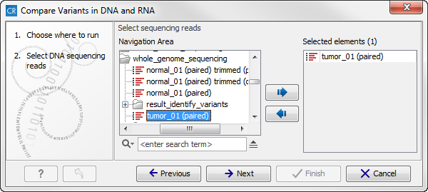
Figure 16.8: Select the DNA reads to analyze. - In the next step you can choose the RNA reads to analyze (see figure 16.9).
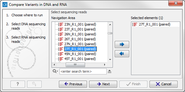
Figure 16.9: Select the RNA reads to analyze. - Click on the button labeled Next to go to the transcriptomic variant detection step (see figure 16.10). For a description of the different parameters that can be adjusted in the variant detection step, we refer to the description of the "Low Frequency Variant Detection" tool in the CLC Cancer Research Workbench user manual (http://www.clcsupport.com/clccancerresearchworkbench/current/index.php?manual=Low_Frequency_Variant_Detection.html). As general filters are applied to the different variant detectors that are available in CLC Cancer Research Workbench, the description of the filters are found in a separate section called "Filters" (see http://www.clcsupport.com/clccancerresearchworkbench/current/index.php?manual=Variant_Detectors_filters.html). If you click on "Locked Settings", you will be able to see all parameters used for variant detection in the ready-to-use workflow.
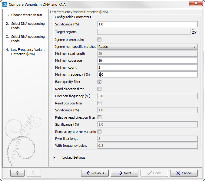
Figure 16.10: Specify the parametes for transcriptomic variant detection. - The next two wizard steps are annotation steps where the transcriptomic variants are annotated with information from known databases. Actually the variants are annotated with a range of different data in this ready-to-use workflow, but only databases that provide data from more than one population needs to be specified by the user. This is the case for HapMap and the 1000 Genomes Project. First, the variants are annotated with information from the 1000 Genomes Project (see figure 16.11). From the drop-down list you can choose the population that matches the population your samples are derived from. The drop-down list shows the populations that were selected under "Data Management" as described in the CLC Cancer Research Workbench user manual (http://www.clcsupport.com/clccancerresearchworkbench/current/index.php?manual=Download_configure_reference_data.html).
Under "Locked settings" you can see that "Automatically join adjacent MNVs and SNVs" has been selected. The reason for this is that many databases do not report a succession of SNVs as one MNV as is the case for the CLC Cancer Research Workbench, and as a consequence it is not possible to directly compare variants called with CLC Cancer Research Workbench with these databases. In order to support filtering against these databases anyway, the option to Automatically join adjacent MNVs and SNVs is enabled. This means that an MNV in the experimental data will get an exact match, if a set of SNVs and MNVs in the database can be combined to provide the same allele.
Note! This assumes that SNVs and MNVs in the track of known variants represent the same allele, although there is no evidence for this in the track of known variants.
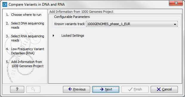
Figure 16.11: Select the relevant population from the drop-down list. - Click on the button labeled Next and do the same to annotate with information from HapMap (figure 16.12).
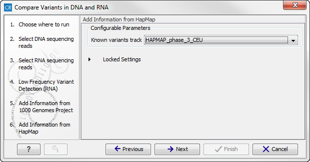
Figure 16.12: Select the relevant population from the drop-down list. - Click on the button labeled Next to go to the genomic variant detection step (shown in figure 16.13).
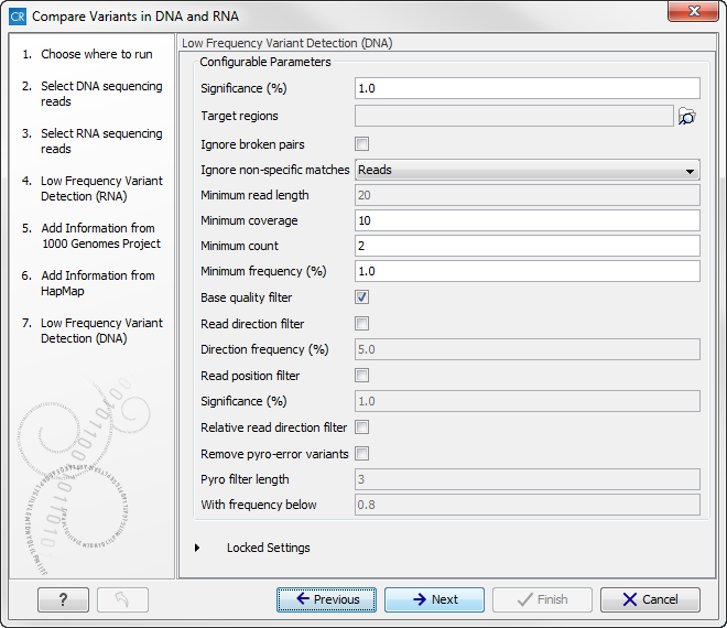
Figure 16.13: Specify the parametes for genomic variant detection. - Again, the two next wizard steps are annotation steps. This time the genomic variants are annotated with information from known databases. First, the variants are annotated with information from the 1000 Genomes Project (see figure 16.14).
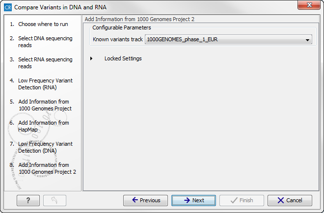
Figure 16.14: Select the relevant population from the drop-down list. - Click on the button labeled Next and do the same to annotate the genomic variants with information from HapMap (figure 16.15).
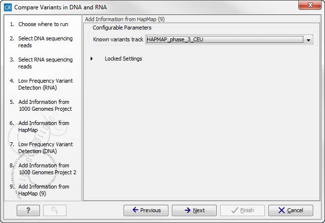
Figure 16.15: Select the relevant population from the drop-down list. - Click on the button labeled Next to go to the result handling step (figure 16.16).
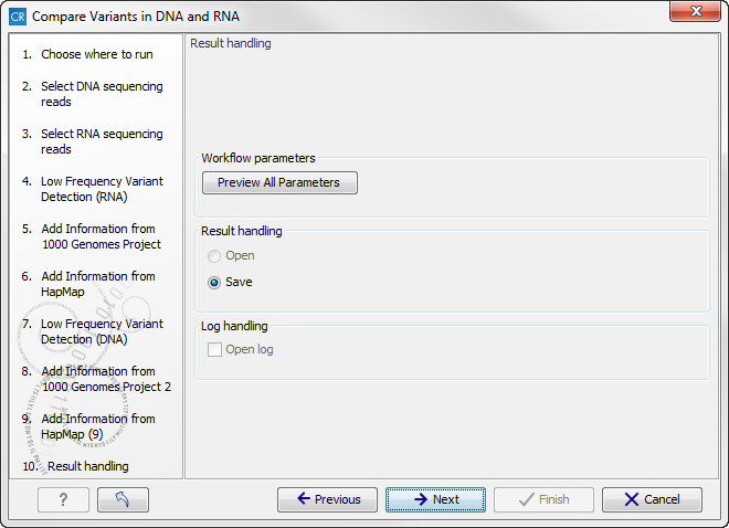
Figure 16.16: Select the relevant population from the drop-down list.Pressing the button Preview All Parameters allows you to preview all parameters. At this step you can only view the parameters, it is not possible to make any changes (see figure 16.17). Choose to save the results and click on the button labeled Finish.
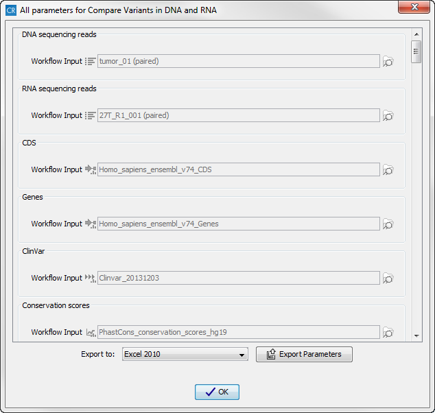
Figure 16.17: Preview all parameters. At this step it is not possible to introduce any changes, it is only possible to view the settings. - Press OK, specify where to save the results, and then click on the button labeled Finish to run the analysis.
Ten different output types are generated:
- DNA Read Mapping (
 ) The mapped DNA sequencing reads. The DNA sequencing reads are shown in different colors depending on their orientation, whether they are single reads or paired reads, and whether they map unambiguously. For the color codes please see the description of sequence colors in the CLC Genomics Workbench manual that can be found here: http://www.clcsupport.com/clcgenomicsworkbench/current/index.php?manual=View_settings_in_Side_Panel.html.
- DNA Mapping Report (
 ) This report contains information about the reads, reference, transcripts, and statistics. This is explained in more detail in the CLC Cancer Research Workbench reference manual in section RNA-Seq report (http://clcsupport.com/clccancerresearchworkbench/current/index.php?manual=RNA_Seq_report.html).
- RNA Gene Expression (
 ) A track showing gene expression annotations. Hold the mouse over or right-clicking on the track. If you have zoomed in to nucleotide level, a tooltip will appear with information about e.g. gene name and expression values.
- RNA Transcript Expression () A track showing transcript expression annotations. Hold the mouse over or right-clicking on the track. A tooltip will appear with information about e.g. gene name and expression values.
- RNA Mapping Report () This report contains information about the reads, reference, transcripts, and statistics. This is explained in more detail in the CLC Cancer Research Workbench reference manual in section RNA-Seq report (http://clcsupport.com/clccancerresearchworkbench/current/index.php?manual=RNA_Seq_report.html).
- RNA Read Mapping () The mapped RNA-seq reads. The RNA-seq reads are shown in different colors depending on their orientation, whether they are single reads or paired reads, and whether they map unambiguously. For the color codes please see the description of sequence colors in the CLC Genomics Workbench manual that can be found here: http://www.clcsupport.com/clcgenomicsworkbench/current/index.php?manual=View_settings_in_Side_Panel.html.
- Variants Found in Both DNA and RNA (
 ) This track shows only the variants that are present in both DNA and RNA. With the table icon (
 ) found in the lower left part of the View Area it is possible to switch to table view. The table view provides details about the variants such as type, zygosity, and information from a range of different databases.
- All Variants Found in DNA or RNA () This track shows all variants that have been detected in either RNA, DNA or both.
- Genome Browser View Variants Found in DNA and RNA (
 ) A collection of tracks presented together. Shows the annotated variants track together with the human reference sequence, genes, transcripts, coding regions, and variants detected in COSMIC, ClinVar and dbSNP (see figure 16.18).
- Log () A log of the workflow execution.
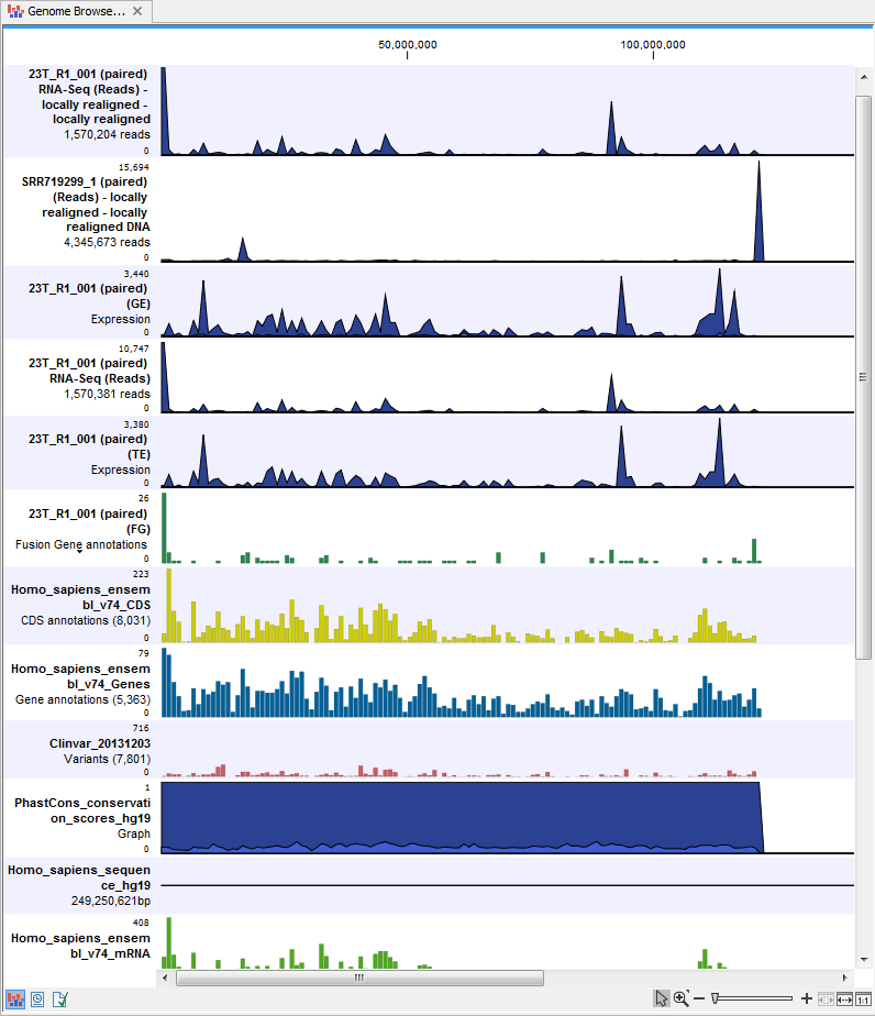
Figure 16.18: The genome browser view makes it easy to compare a range of different data.
The three most important tracks of the ten generated are the Variants found in both DNA and RNA track, All variants found in DNA or RNA track, and the Genome Browser View. The Genome Browser View makes it easy to get an overview in the context of a reference sequence, and compare variant and expression tracks with information from different databases. The two other tracks (Variants found in both DNA and RNA track and All variants found in DNA or RNA track) provides detailed information about the detected variants when opened in table view.