References
The second section of the detailed report concerns the Reference sequence(s).
First, a table gives information about Reference coverage, including coverage statistics and GC content of the reference sequence.
The second table gives Coverage statistics. A position on the reference is counted as "covered" when at least one read is aligned to it. Note that unaligned ends (faded nucleotides at the ends) that are produced when mapping using local alignment do not contribute to the coverage. Also, positions with an ambiguous nucleotide in the reference (i.e., not A, C, T or G) count as zero coverage regions, regardless of the number of reads mapping across them.
In the example shown in figure 26.13, there is a region of zero coverage in the middle and one time coverage on each side. Note that the gaps to the very right are within the same read which means that these two positions on the reference sequence are still counted as "covered".
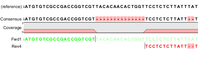
Figure 26.13: A region of zero coverage in the middle and one time coverage on each side. Note that the gaps to the very right are within the same read which means that these two positions on the reference sequence are still counted as "covered".
In this table, coverage is reported on two levels: including and excluding zero coverage regions. In some cases, you do not expect the whole reference to be covered, and only the coverage levels of the covered parts of the reference sequence are interesting. On the other hand, if you have sequenced the full genome that you use as reference, the overall coverage is probably the most relevant number (i.e. including zero coverage regions).
In the third and fourth subsections, two graphs display Coverage level distribution, with and without zero coverage regions. Two bar plots show the distribution of coverage with coverage level on the x-axis and number of positions with that coverage on the y-axis (as seen in figure 26.14).
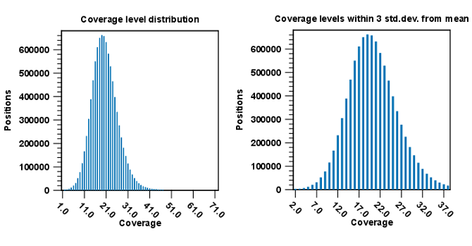
Figure 26.14: Distribution of coverage - to the left for all the coverage levels, and to the right for coverage levels within 3 standard deviations from the mean.
The graph to the left shows all the coverage levels, whereas the graph to the right shows coverage levels within 3 standard deviations from the mean. The reason for this is that for complex genomes, you will often have a few regions with extremely high coverage which will affect the resolution of the graph, making it impossible to see the coverage distribution for the majority of the references. These coverage outliers are excluded when only showing coverage within 3 standard deviations from the mean. Below the second coverage graph there are some statistics on the data that is outside the 3 standard deviations.
Subsection 5 gives some statistics on the Zero coverage regions; the number, minimum and maximum length, mean length, standard deviation, and total length.
One of the biases seen in sequencing data concerns GC content. Often there is a correlation between GC content and coverage. In order to investigate this correlation, the report includes in subsection 6 a Coverage versus GC Content graph plotting coverage against GC content (see figure 26.15). Note that you can see the GC content for each reference sequence in the table(s) above.
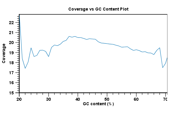
Figure 26.15: The plot displays, for each GC content level (0-100 %), the mean read coverage of 100bp reference segments with that GC content.
The plot displays, for each GC content level (0-100 %), the mean read coverage of 100bp reference segments with that GC content.
For a report created from a de novo assembly, this section finishes with statistics about the reads which are the same for both reference and de novo assembly (see Read statistics).