Identify Enriched Variants in Case vs Control Samples
This tool should be used if you have a case-control study. This could be individuals with a disease (case) and healthy individuals (control). The Identify Enriched Variants in Case vs Control Samples tool will identify variants that are significantly more common in the case samples than in the control samples. The Fisher exact test is applied on the number of occurrences of each allele of each variant in the case and the control data set. The alleles from each variant are considered separately, i.e. for an SNV with two alleles; a Fisher Exact test will be applied to each of the two. The test will also check whether an SNV in the case group is part of an MNV in the control group. Those with a low p-value are potential candidates for variants playing a role in the disease/phenotype. Please note that a low p-value can only be reached if the number of samples in the data set is high.
Toolbox | Resequencing Analysis (![]() ) | Variants Comparison (
) | Variants Comparison (![]() ) | Identify Enriched Variants in Case vs Control Samples (
) | Identify Enriched Variants in Case vs Control Samples (![]() )
)
In the first step of the dialog, you select the case variant tracks (figure 29.10).
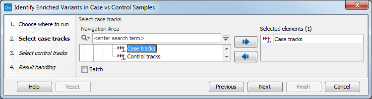
Figure 29.10: Select the case variant track.
Clicking Next shows the dialog in figure 29.11.
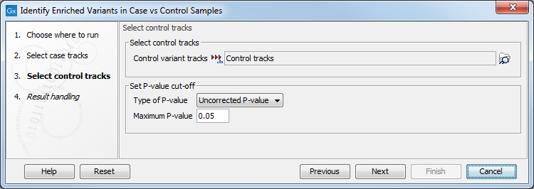
Figure 29.11: In this dialog you can select the control tracks, a p-value correction method, and specify the p-value threshold for the fisher exact test.
At the top, select the variant tracks from the control group. Furthermore, you must set a threshold for the p-value (default is 0.05); only variants having a p-value below this threshold will be reported. You can choose whether the threshold p-value refers to a corrected value for multiple tests (either Bonferroni Correction, or False Discovery Rate (FDR)), or an uncorrected p-value. A variant table is created as output (see figure 29.12), reporting only those variants with p-values lower than the threshold. All corrected and uncorrected p-values are shown here, so alternatively, variants with non-significant p-values can also be filtered out or more stringent thresholds can be applied at this stage, using the manual filtering options.
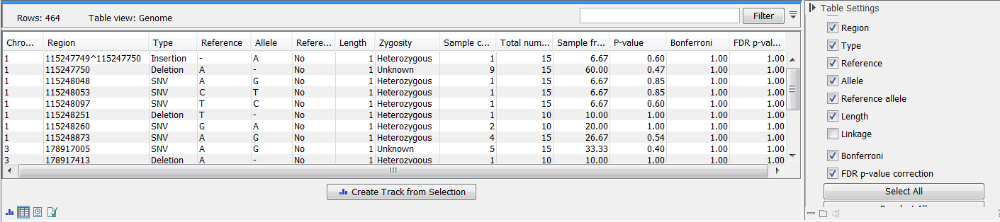
Figure 29.12: In the output table, you can view information about all significant variants, select which columns to view, and filter manually on certain criteria.
There are many other columns displaying information about the variants in the output table, such as the type, sequence, and length of the variant, its frequency and read count in case and control samples, and its overall zygosity. The zygosity information refers to all of the case samples; a label of 'homozygous' means the variant is homozygous in all case samples, a label of 'heterozygous' means the variant is heterozygous in all case samples, whereas a label of 'unknown' means it is heterozygous in some, and homozygous in others.
Overlapping variants: If two different types of variants occur in the same location, these are reported separately in the output table. This is particularly important, where SNPs occur in the same position as an MNV. Usually, multiple SNVs occurring alongside each other would simply be reported as one MNV, but if one SNV of the MNV is found in additional case samples by itself, it will be reported separately. For example, if an MNV of AAT -> GCA at position 1 occurs in five of the case samples, and the SNV at position 1 of A -> G, occurs in an additional 3 samples (so 8 samples in total), the output table will list the MNV and SNV information separately (however, the SNV will be shown as being present in only 3 samples, as this is the number in which it appears 'alone').
The test will also check whether an SNV in the case group is part of an MNV in the control group.