The EM estimation algorithm
The EM estimation algorithm is inspired by the RSEM and eXpress methods. It iteratively estimates the abundance of transcripts, and assigns reads to transcripts according to these abundances. To illustrate the interpretation of `transcript abundance', consider the following two examples.
In the first example, we have a gene with two transcripts, where one transcript is twice as long as the other (figure 26.8). This longer transcript is also twice as abundant, meaning that in the exon common to both transcripts two of the three reads come from the longer transcript, and the final read comes from the shorter transcript. The longer transcript has a second exon which also generates two reads. We see then that the longer transcript is twice as abundant, but because it is twice as long it generates four times as many reads.
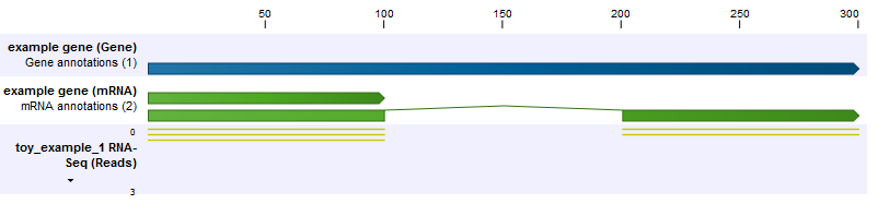
Figure 26.8: The longer transcript has twice the abundance, but four times the number of reads as the shorter transcript.
In the second example, the set up is the same, but now the shorter transcript is twice as abundant as the longer transcript (figure 26.9). Because the longer transcript is twice as long, there are equal numbers of reads from each transcript.
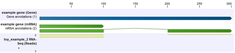
Figure 26.9: The longer transcript has half the abundance, but the same number of reads as the shorter transcript.
To estimate the transcript abundances, we carry out an expectation-maximization procedure. Before explaining the procedure, first we define the concept of a mapping. A mapping is a set of transcripts, to which a read may map. In the above examples, some reads have the mapping
![]() (these are non-uniquely mapping reads), and some reads have the mapping
(these are non-uniquely mapping reads), and some reads have the mapping
![]() (these are `uniquely' mapping reads). In both examples, the count of mapping
(these are `uniquely' mapping reads). In both examples, the count of mapping ![]() is 3, because there are 3 shared reads between the transcripts. The count of mapping
is 3, because there are 3 shared reads between the transcripts. The count of mapping ![]() is 2 in the first example, and 1 in the second example.
is 2 in the first example, and 1 in the second example.
The expectation-maximization algorithm proceeds as follows:
- The transcript abundances are initialized to the uniform distribution, i.e. at the start all transcripts are assumed to be equally expressed.
- Expectation step: the current (assumed) transcript abundances are used to calculate the expected count of each transcript, i.e. the number of reads we expect should be assigned to the given transcript. This is done by looping over all mappings that include the given transcript, and assigning a proportion of the total count of that mapping to the transcript. The proportion corresponds to the proportion of the total transcript abundance in the mapping that is due to the target.
- Maximization step: the currently assigned counts of each transcript are used to re-compute the transcript abundances. This is done by looping over all targets, and for each target, dividing the proportion of currently assigned counts for the transcript (=total counts for transcript/total number of reads) by the target length. This is necessary because longer transcripts are expected to generate proportionally more reads.
- Repeat from step 2 until convergence.
Below, we illustrate how the expectation-maximization algorithm converges to the expected abundances for the above two examples.
Example 1:
Initially: transcript 2 abundance = 0.50, count: 0.00, transcript 1 abundance = 0.50, count: 0.00
After 1 round: transcript 2 abundance = 0.54, count: 3.50, transcript 1 abundance = 0.46, count: 1.50
After 2 rounds: transcript 2 abundance = 0.57, count: 3.62, transcript 1 abundance = 0.43, count: 1.38
After 3 rounds: transcript 2 abundance = 0.59, count: 3.70, transcript 1 abundance = 0.41, count: 1.30
After 4 rounds: transcript 2 abundance = 0.60, count: 3.76, transcript 1 abundance = 0.40, count: 1.24
After 5 rounds: transcript 2 abundance = 0.62, count: 3.81, transcript 1 abundance = 0.38, count: 1.19
After 6 rounds: transcript 2 abundance = 0.62, count: 3.85, transcript 1 abundance = 0.38, count: 1.15
After 7 rounds: transcript 2 abundance = 0.63, count: 3.87, transcript 1 abundance = 0.37, count: 1.13
After 8 rounds: transcript 2 abundance = 0.64, count: 3.90, transcript 1 abundance = 0.36, count: 1.10
After 9 rounds: transcript 2 abundance = 0.64, count: 3.92, transcript 1 abundance = 0.36, count: 1.08
After 10 rounds: transcript 2 abundance = 0.65, count: 3.93, transcript 1 abundance = 0.35, count: 1.07
After 11 rounds: transcript 2 abundance = 0.65, count: 3.94, transcript 1 abundance = 0.35, count: 1.06
After 12 rounds: transcript 2 abundance = 0.65, count: 3.95, transcript 1 abundance = 0.35, count: 1.05
After 13 rounds: transcript 2 abundance = 0.66, count: 3.96, transcript 1 abundance = 0.34, count: 1.04
After 14 rounds: transcript 2 abundance = 0.66, count: 3.97, transcript 1 abundance = 0.34, count: 1.03
After 15 rounds: transcript 2 abundance = 0.66, count: 3.97, transcript 1 abundance = 0.34, count: 1.03
Example 2:
Initially: transcript 2 abundance = 0.50, count: 0.00, transcript 1 abundance = 0.50, count: 0.00
After 1 round: transcript 2 abundance = 0.45, count: 2.50, transcript 1 abundance = 0.55, count: 1.50
After 2 rounds: transcript 2 abundance = 0.42, count: 2.36, transcript 1 abundance = 0.58, count: 1.64
After 3 rounds: transcript 2 abundance = 0.39, count: 2.26, transcript 1 abundance = 0.61, count: 1.74
After 4 rounds: transcript 2 abundance = 0.37, count: 2.18, transcript 1 abundance = 0.63, count: 1.82
After 5 rounds: transcript 2 abundance = 0.36, count: 2.12, transcript 1 abundance = 0.64, count: 1.88
After 6 rounds: transcript 2 abundance = 0.35, count: 2.08, transcript 1 abundance = 0.65, count: 1.92
After 7 rounds: transcript 2 abundance = 0.35, count: 2.06, transcript 1 abundance = 0.65, count: 1.94
After 8 rounds: transcript 2 abundance = 0.34, count: 2.04, transcript 1 abundance = 0.66, count: 1.96
After 9 rounds: transcript 2 abundance = 0.34, count: 2.03, transcript 1 abundance = 0.66, count: 1.97
After 10 rounds: transcript 2 abundance = 0.34, count: 2.02, transcript 1 abundance = 0.66, count: 1.98
After 11 rounds: transcript 2 abundance = 0.34, count: 2.01, transcript 1 abundance = 0.66, count: 1.99
After 12 rounds: transcript 2 abundance = 0.34, count: 2.01, transcript 1 abundance = 0.66, count: 1.99
After 13 rounds: transcript 2 abundance = 0.33, count: 2.01, transcript 1 abundance = 0.67, count: 1.99
After 14 rounds: transcript 2 abundance = 0.33, count: 2.00, transcript 1 abundance = 0.67, count: 2.00
After 15 rounds: transcript 2 abundance = 0.33, count: 2.00, transcript 1 abundance = 0.67, count: 2.00
Once the algorithm has converged, every non-uniquely mapping read is assigned randomly to a particular transcript according to the abundances of transcripts within the same mapping. The total transcript reads column reflects these assignments. The RPKM and TPM values are then computed from the counts assigned to each transcript.