Feature selection and dimensionality reduction
Several tools provide options for speeding up calculations and reducing noise by decreasing the amount of data used. The available options are:
- Feature selection, where only highly variable genes (HVGs) are used.
- Dimensionality reduction, where data is projected into a lower dimensional space, through either principal component analysis (PCA) for expression data, or latent semantic indexing (LSI) for peak data.
Highly variable genes (HVGs)
Not all genes are equally informative when clustering or visualizing cells. For example, housekeeping genes, whose expression levels are approximately constant across different cell types, are not informative for distinguishing between cell types. It is therefore often possible to get qualitatively the same results from an analysis by only using genes whose expression levels are highly variable across cells.
In order to use HVGs, data must first have been normalized by Normalize Single Cell Data. Use highly variable genes is not selected by default, but may be appropriate when speed is a priority, or when results using all genes appear unsatisfactory. The Number of highly variable genes to use must be specified. Values in the range ![]() -
-![]() are typically sufficient to capture most variation from most data sets. Setting this value too low may exclude genes that are weakly informative, such as those that have small fold changes in rare cell types.
are typically sufficient to capture most variation from most data sets. Setting this value too low may exclude genes that are weakly informative, such as those that have small fold changes in rare cell types.
|
Highly variable peaks HVGs can only be used for expression data, and not for peak data. The only exception to this is when a tool works with expression and peak data simultaneously, and where no dimensionality reduction is applied. In this case, which is not recommended, the same number of peaks as HVGs are chosen at random to be "highly variable peaks". |
When a tool is run, the log will contain estimates of the amount of signal and noise removed by choosing a certain number of HVGs (figure 14.1), which may help when choosing an appropriate value.
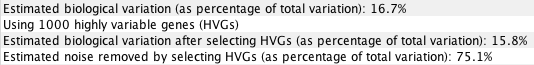
Figure 14.1: An example of information provided in a tool log. Here, using ![]() HVGs reduced the total amount of variation in the data. However, the majority of the removed variation was estimated to be noise (
HVGs reduced the total amount of variation in the data. However, the majority of the removed variation was estimated to be noise (![]() of the original variation) and only a small amount of signal was lost (
of the original variation) and only a small amount of signal was lost (
![]() of the original variation). For more details on variation estimates, see Calculation of estimated biological variation.
of the original variation). For more details on variation estimates, see Calculation of estimated biological variation.
Genes are selected to be HVGs according to the variance of their normalized values, from highest variance to lowest variance. Genes with variance ![]() are never selected, as this is consistent with random noise - this means that the number of HVGs used in an analysis may be lower than the number specified.
are never selected, as this is consistent with random noise - this means that the number of HVGs used in an analysis may be lower than the number specified.
Note that using HVGs in one part of an analysis does not limit the number of genes available in downstream steps. For example, after constructing a visualization with HVGs, it is still possible to visualize the expressions of all genes.
Dimensionality reduction by PCA or LSI
In most circumstances it is recommended to Use dimensionality reduction as it provides a substantial increase in speed without affecting accuracy. Exceptions might include analysis of targeted expression data, where the expression of only a few hundred genes is measured.
Dimensionality reduction is by PCA for expression data, and LSI for peak data, using ![]() number of dimensions as set in the Dimensions option. When both data types are present,
number of dimensions as set in the Dimensions option. When both data types are present, ![]() PCA components and
PCA components and ![]() LSI components are used, and each cell is represented by 2 *
LSI components are used, and each cell is represented by 2 * ![]() features.
features.
Principal Component Analysis (PCA)
Principal Component Analysis (PCA) projects data into a lower dimensional space while preserving as much variation as possible.
Not all PCA dimensions are equal - the first dimension contains most of the variation and each subsequent dimension contains less of the variation than the previous one. For this reason, it often makes little difference to results whether ![]() is set to
is set to ![]() or
or ![]() , but large differences can be observed if too few PCA dimensions are used. Values in the range
, but large differences can be observed if too few PCA dimensions are used. Values in the range ![]() -
-![]() are suitable for most applications. If the data has been normalized by Normalize Single Cell Data, the log will contain estimates of the amount of biological variation in the data, which can be compared to the amount of variation captured by the chosen number of PCA dimensions (figure 14.2). For details on how biological variation is estimated, see Calculation of estimated biological variation.
are suitable for most applications. If the data has been normalized by Normalize Single Cell Data, the log will contain estimates of the amount of biological variation in the data, which can be compared to the amount of variation captured by the chosen number of PCA dimensions (figure 14.2). For details on how biological variation is estimated, see Calculation of estimated biological variation.
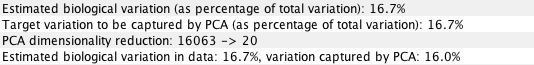
Figure 14.2: An example of information provided in a tool log. Here, using ![]() PCA dimensions captured
PCA dimensions captured ![]() of variation in the data. This is comparable with the estimated amount of biological variation in the data.
of variation in the data. This is comparable with the estimated amount of biological variation in the data.
PCA is performed using an implementation of Algorithm 971 [Li et al., 2017]. This is an extremely fast and accurate algorithm for finding the first PCA dimensions, but its accuracy decreases for higher dimensions. For this reason, it is advised to keep the number of PCA dimensions small compared to the number of expressed genes.
When data have been normalized by Normalize Single Cell Data it is additionally possible to Automatically select PCA dimensions. This chooses a number of dimensions ![]() that contain the same amount of variation as the estimated biological variation. An example log is shown in figure 14.3.
that contain the same amount of variation as the estimated biological variation. An example log is shown in figure 14.3.
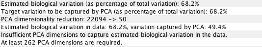
Figure 14.3: An example of information provided in a tool log when selecting PCA dimensions automatically. Here, using ![]() PCA dimensions captured
PCA dimensions captured ![]() of variation in the data, which was lower than the estimated biological (i.e. non-noise) variation in the data. At least
of variation in the data, which was lower than the estimated biological (i.e. non-noise) variation in the data. At least ![]() PCA dimensions are required to capture all
PCA dimensions are required to capture all ![]() of the variation estimated to be biological. However, the estimates are upper bounds and in practice
of the variation estimated to be biological. However, the estimates are upper bounds and in practice ![]() dimensions is likely to be sufficient.
dimensions is likely to be sufficient.
Latent Semantic Indexing (LSI)
Latent Semantic Indexing (LSI) is often applied in natural language processing to a "document-term" matrix, which tabulates the number of times different words (terms) are seen in different documents. The technique returns a lower-dimensional representation of the matrix, with a reduced number of terms. These terms are linear combinations of original terms that are often found in the same documents.
In the context of scATAC-Seq, the peaks are terms and the cells are documents. The reduced dimensions are therefore linear combinations of peaks that are often found in groups of cells.
We construct a "document-term" matrix from the Peak Count Matrix using a Term Frequency - Inverse Document Frequency (TF-IDF) weighting:
Here ![]() is the number of cells,
is the number of cells, ![]() is the Peak Count Matrix element for cell
is the Peak Count Matrix element for cell ![]() and peak
and peak ![]() ,
,
![]() is the indicator function that returns
is the indicator function that returns ![]() if
if
![]() or else 0, and
or else 0, and
![]() is the number of cells containing peak
is the number of cells containing peak ![]() .
.
LSI with ![]() dimensions is then achieved by taking the first
dimensions is then achieved by taking the first ![]() -components of the
-components of the
![]() matrix returned by singular value decomposition of
matrix returned by singular value decomposition of
![]() :
:
To correct for the effect of sequencing depth, the
![]() matrix is re-normalized such that each cell is represented by a unit vector:
matrix is re-normalized such that each cell is represented by a unit vector:

Combining HVGs and PCA or LSI
It is possible to use HVGs and dimensionality reduction together. When this is done, HVGs are selected and then dimensionality reduction is run only on the HVGs. Note that, because using HVGs already removes a lot of noise, the log may show that even a relatively large number of Dimensions is insufficient to capture all the estimated biological variation. It may be worth experimenting with increasing the number of dimensions slightly to check whether this has an impact on the results.
Using both expression and peak data
When feature selection and/or dimensionality reduction is applied to both an expression and peak matrix, only cells that are in common to both matrices are used.
It is possible to run only feature selection without dimensionality reduction. To ensure that the two data types contribute equally to the downstream analysis, the number of peaks is also reduced to the same number as the genes. Since no corresponding method for feature selection exists for peak data, the peaks are chosen randomly.
When dimensionality reduction is applied, all peaks are used, regardless of the HVGs settings, as the dimensionality reduction ensures equal contribution of both data types.
Subsections