Running the Empirical analysis of DGE
First, find the Empirical analysis of DGE tool:
Toolbox | Microarray and Small RNA Analysis (![]() )| Statistical Analysis | Empirical Analysis of DGE (
)| Statistical Analysis | Empirical Analysis of DGE (![]() )
)
The original count data for a full expression experiment are the expected input to the Empirical Analysis of DGE tool.
When Experiments created within the Workbench are used as input, the original count values are always used. Columns of such Experiments that contain transformed or normalized values are ignored.
If expression values are being imported from outside the Workbench for use with this test, the data should be original (non-transformed, non-normalized) counts.
Whether the data has been generated in the Workbench or outside the Workbench and imported, the full set of expression results should be used. Please do not run this test on a subset of values from the original sample data.
The reason that the complete set of original count data for samples should be used as input to this test is that the algorithm assumes that the counts on which it operates are Negative Binomially distributed. It implicitly normalizes and transforms these counts, so if the counts have been altered prior to submitting them to the Empirical Analysis of DGE tool, this assumption is likely to be compromised.
When running the Empirical analysis of DGE tool in the Genomics workbench, the user is asked to specify two parameters related to the estimation of the dispersion (figure 29.57). Of these, the 'Total count filter cut-off' specifies which features should be considered when estimating the common dispersion component. Features for which the counts across all samples are low are likely to contribute mostly with noise to the estimation, and features with a lower cummulative count across samples than the value specified will be ignored. When the check-box 'Estimate tag-wise dispersions' is checked, the dispersion estimate for each gene will be a weighted combination of the tag-wise and common dispersion, if the check-box is un-ticked the common dispersion will be used for all genes.
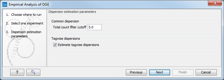
Figure 29.57: Empirical analysis of DGE: setting the parameters related to dispersion.
The Empirical analysis of DGE may be carried out between all pairs of groups (by clicking the 'All pairs' button) or for each group against a specified reference group (by clicking the 'Against reference' button) (figure 29.58). In the last case you must specify which of the groups you want to use as reference (the default is to use the group you specified as Group 1 when you set up the experiment). Foe example, the All pairs option should be selected when you wish to perform the test of equality for group means for all of the pairs, e.g. if you would like to compare different tissues where each tissue is represented in a group. In this case there is no reference group, so the following comparisons will be performed:
- liver vs heart
- liver vs lung
- heart vs lung
- Wild type vs Mutant 1
- Wild type vs Mutant 2
Below you can select to add two kinds of corrected p-values to the analysis (in addition to the standard p-value produced for the test statistic):
- Bonferroni corrected.
- FDR corrected.
The Bonferroni corrected p-values handle the multiple testing problem by controlling the 'family-wise error rate': the probability of making at least one false positive call. They are calculated by multiplying the original p-values by the number of tests performed. The probability of having at least one false positive among the set of features with Bonferroni corrected p-values below 0.05, is less than 5%. The Bonferroni correction is conservative: there may be many genes that are differentially expressed among the genes with Bonferroni corrected p-values above 0.05, that will be missed if this correction is applied.
Instead of controlling the family-wise error rate we can control the false discovery rate: FDR. The false discovery rate is the proportion of false positives among all those declared positive. We expect 5 % of the features with FDR corrected p-values below 0.05 to be false positive. There are many methods for controlling the FDR - the method used in CLC Genomics Workbench is that of [Benjamini and Hochberg, 1995].
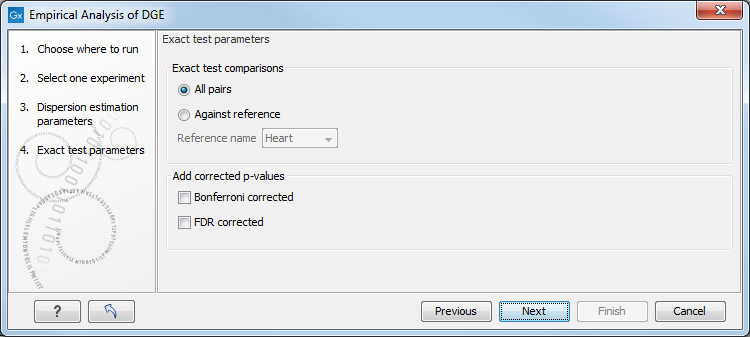
Figure 29.58: Empirical analysis of DGE: setting comparisons and corrected p-value options.
When the Empirical analysis of DGE is run three columns will be added to the experiment table for each pair of groups that are analyzed: the 'P-value', 'Fold change' and 'Weighted difference' columns. The 'P-value' holds the p-value for the Exact test. The 'Fold Change' and 'Weighted difference' columns are both calculated from the estimated relative abundances, which are derived internally in the Exact Test algorithm. They depend on both the sizes (depth of coverage/library size) of the samples, the magnitude of the counts and on the estimated negative binomial dispersion, so they cannot be obtained from the original counts by simple algebraic calculations.
The 'Fold Change' will tell you how many times bigger the relative abundance of group 2 is relative to that of group 1. If the relative abundance of group 2 is bigger than that of group 1 the fold change is the relative abundance of group 2 divided by that of group 1. If the relative abundance of group 2 is smaller than that of group 1 the fold change is the relative abundance of group 1 divided by that of group 2 with a negative sign. The 'weighted difference' column contains the difference between the relative abundance of group 2 and the relative abundance of group 1. In addition to the three automatically added columns, columns containing the Bonferroni and FDR corrected p-values will be added if that was specified by the user.