Map to Specified Reference
Once analysis has been performed using the Type Among Multiple Species workflow, the best matching reference is listed in the Result Metadata table (figure 3.45, see column Best match).
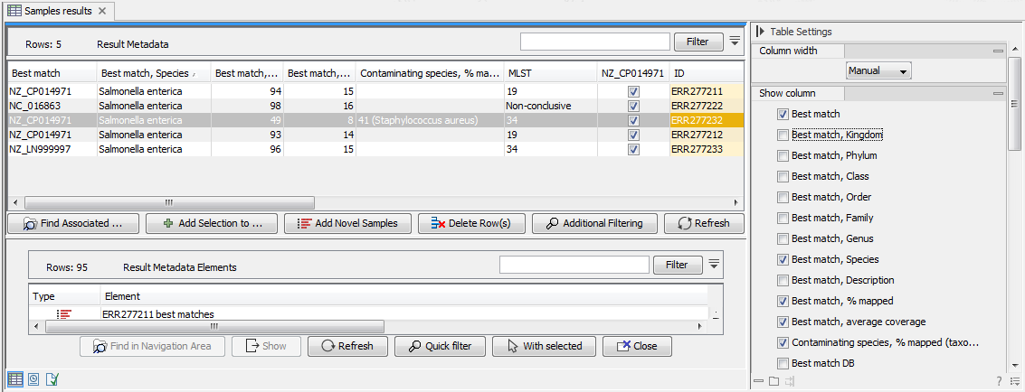
Figure 3.45: Best match references are listed for each row in the Result Metadata Table.
If all your samples share the same common reference, you can proceed to additional analyses without delay.
However there are cases where your samples have different Best match reference for a particular MLST scheme. And because creating a SNP Tree require a single common reference, you will need to identify the best matching common reference for all your samples using a K-mer Tree, as well as subsequently re-map your samples to this common reference.
If you already know the common reference for the sample you want to use to create a SNP tree, you can directly specify that reference in the re-map workflow. Otherwise, finding a common reference is described in more details in section 10.2.
In short, to identify a common reference across multiple clades within the Result Metadata Table:
- Select samples to which a common best matching references should be identified.
- Click on the Find Associated Data (
 ) button to find their associated Metadata Elements.
- Click on the Quick Filtering (
 ) button and select the option Filter for K-mer Tree to find Metadata Elements with the Role = Trimmed Reads.
- Select the relevant Metadata Element files.
- Click on the With selected (
 ) button.
- Select the Create K-mer Tree action and follow the wizard as described in the section called Create K-mer Tree.
The common reference, chosen as sharing the closest common ancestor with the clade of isolates under study in the k-mer tree, is subsequently used as a reference for the Map to Specified Reference workflow (figure 3.46) that will perform a re-mapping of the reads followed by variant calling.
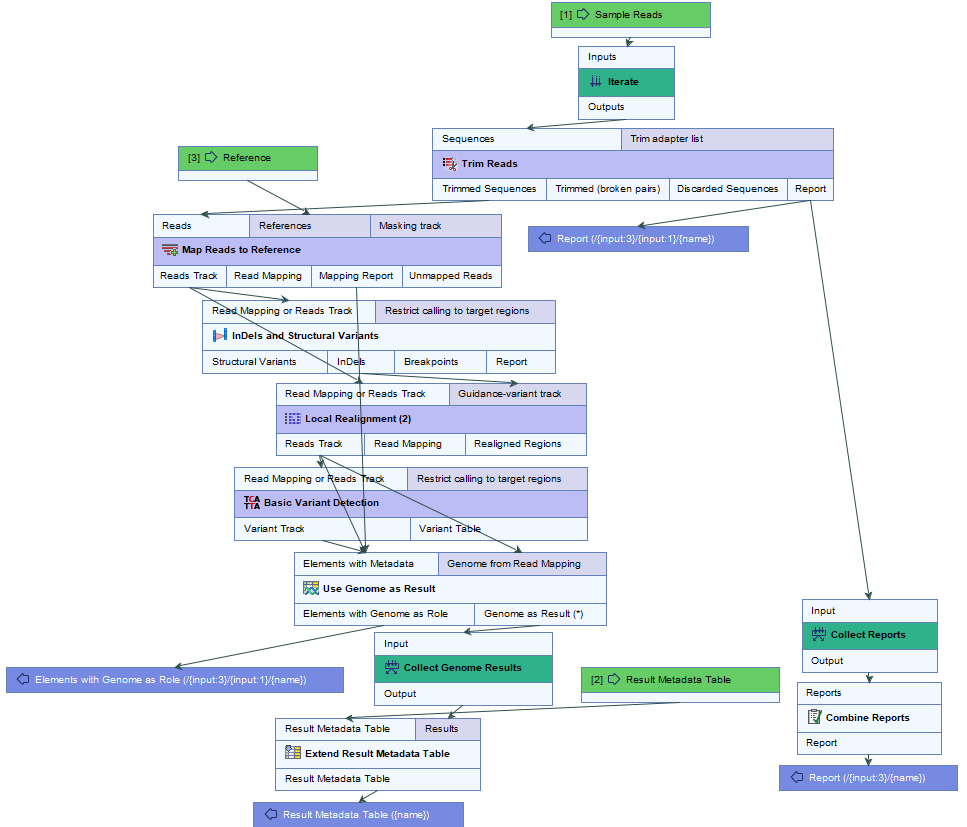
Figure 3.46: Overview of the template Map to Specified Reference workflow.
How to run the Map to Specified Reference workflow
This workflow is intended for read mapping and variant calling of the samples to a common reference. To run the workflow, go to:
Toolbox | Template Workflows (![]() ) | Microbial Workflows (
) | Microbial Workflows (![]() ) | Typing and Epidemiology (
) | Typing and Epidemiology (![]() ) | Map to Specified Reference (
) | Map to Specified Reference (![]() )
)
- Specify the sample(s) or folder(s) of samples you would like to type (figure 3.47) and click Next. Remember that if you select several items, they will be run as batch units.
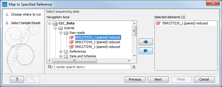
Figure 3.47: Select the reads from the sample(s) you would like to type. - Specify the Result Metadata Table you want to use (figure 3.48) and click Next.
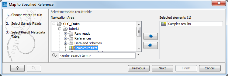
Figure 3.48: Select the metadata table you would like to use. - Select the reference you obtained from the previous workflows - provided that it was the same reference for all the samples you want to re-map - or determined earlier from your K-mer tree if the samples you want to re-map had different best match references. Click Next.
- Define batch units using organisation of input data to create one run per input or use a metadata table to define batch units. Click Next.
- The next wizard window gives you an overview of the samples present in the selected folder(s). Choose which of these samples you want to analyze in case you are not interested in analyzing all the samples from a particular folder (figure 3.49).
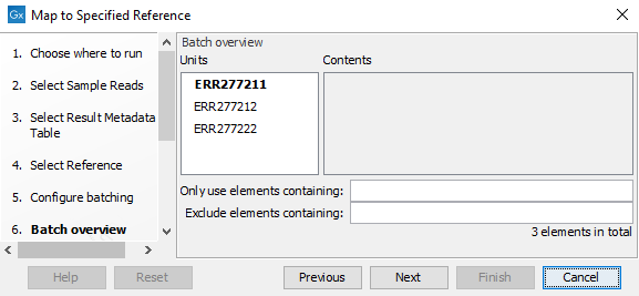
Figure 3.49: Choose which of the samples present in the selected folder(s) you want to analyze. - You can specify a trim adapter list and set up parameters if you would like to trim your sequences from adapters. Specifying a trim adapter list is optional but recommended to ensure the highest quality data for your typing analysis (figure 3.50). Learn about trim adapter lists at http://resources.qiagenbioinformatics.com/manuals/clcgenomicsworkbench/current/index.php?manual=Trim_adapter_list.html.
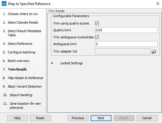
Figure 3.50: You can choose to trim adapter sequences from your sequencing reads.The parameters that can be set are:
- Ambiguous trim: if checked, this option trims the sequence ends based on the presence of ambiguous nucleotides (typically N).
- Ambiguous limit: defines the maximal number of ambiguous nucleotides allowed in the sequence after trimming.
- Quality trim: if checked, and if the sequence files contain quality scores from a base-caller algorithm, this information can be used for trimming sequence ends.
- Quality limit: defines the minimal value of the Phred score for which bases will not be trimmed.
- Specify the parameters for the Maps Reads to Reference tool (figure 3.51).
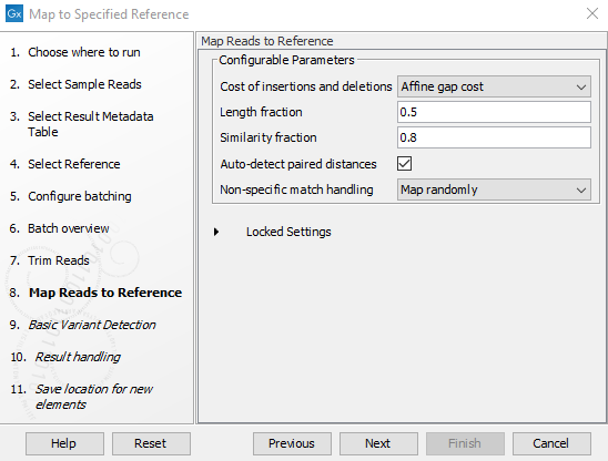
Figure 3.51: Specify the parameters for the Maps Reads to Reference tool.The parameters that can be set are:
- Cost of insertion and deletions: You can choose affine or linear gap cost.
- Length fraction: The minimum percentage of the total alignment length that must match the reference sequence at the selected similarity fraction. A fraction of 0.5 means that at least half of the alignment must match the reference sequence before the read is included in the mapping (if the similarity fraction is set to 1). Note that the minimal seed (word) size for read mapping is 15 bp, so reads shorter than this will not be mapped.
- Similarity fraction: The minimum percentage identity between the aligned region of the read and the reference sequence. For example, if the identity should be at least 80% for the read to be included in the mapping, set this value to 0.8. Note that the similarity fraction relates to the length fraction, i.e., when the length fraction is set to 50% then at least 50% of the alignment must have at least 80% identity
- Auto-detect paired sequences: This will determine the paired distance (insert size) of paired data sets. If several paired sequence lists are used as input, a separate calculation is done for each one to allow for different libraries in the same run.
- Non-specific match handling: You can choose from the drop down menu whether you would like to ignore or map randomly the non specific matches.
- Specify the parameters for the Basic Variant Detection tool (figure 3.52) before clicking Next.
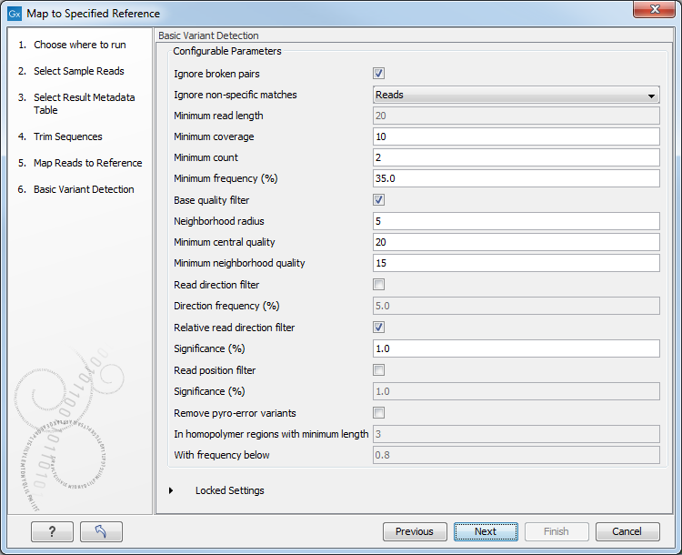
Figure 3.52: Specify the parameters to be used for the Basic Variant Detection tool.The parameters that can be set are:
- Ignore broken pairs: You can choose to ignore broken pairs by clicking this option.
- Ignore non-specific matches: You can choose to ignore non-specific matches between reads, regions or to not ignore them at all.
- Minimum read length: Only variants in reads longer than this size are called.
- Minimum coverage: Only variants in regions covered by at least this many reads are called.
- Minimum count: Only variants that are present in at least this many reads are called.
- Minimum frequency %: Only variants that are present at least at the specified frequency (calculated as count/coverage) are called.
- Base quality filter: The base quality filter can be used to ignore the reads whose nucleotide at the potential variant position is of dubious quality.
- Neighborhood radius: Determine how far away from the current variant the quality assessment should extend.
- Minimum central quality: Reads whose central base has a quality below the specified value will be ignored. This parameter does not apply to deletions since there is no "central base" in these cases.
- Minimum neighborhood quality: Reads for which the minimum quality of the bases is below the specified value will be ignored.
- Read direction filters: The read direction filter removes variants that are almost exclusively present in either forward or reverse reads.
- Direction frequency %: Variants that are not supported by at least this frequency of reads from each direction are removed.
- Relative read direction filter: The relative read direction filter attempts to do the same thing as the Read direction filter, but does this in a statistical, rather than absolute, sense: it tests whether the distribution among forward and reverse reads of the variant carrying reads is different from that of the total set of reads covering the site. The statistical, rather than absolute, approach makes the filter less stringent.
- Significance %: Variants whose read direction distribution is significantly different from the expected with a test at this level, are removed. The lower you set the significance cut-off, the fewer variants will be filtered out.
- Read position filter: It removes variants that are located differently in the reads carrying it than would be expected given the general location of the reads covering the variant site.
- Significance %: Variants whose read position distribution is significantly different from
the expected with a test at this level, are removed. The lower you set the significance
cut-off, the fewer variants will be filtered out.
- Remove pyro-error variants: This filter can be used to remove insertions and deletions in the reads that are likely to be due to pyro-like errors in homopolymer regions. There are two parameters that must be specified for this filter:
- In homopolymer regions with minimum length: Only insertion or deletion variants in homopolymer regions of at least this length will be removed.
- With frequency below: Only insertion or deletion variants whose frequency (ignoring all non-reference and non-homopolymer variant reads) is lower than this threshold will be removed.
- In the Result handling window, pressing the button Preview All Parameters allows you to preview - but not change - all parameters. Choose to save the results and click on the button labeled Finish.
Four outputs are generated per input sample (figure 3.53):

Figure 3.53: Output files from the Map to Specified Reference workflow.
- Mapping Summary report: summary report about the mapping process, see http://resources.qiagenbioinformatics.com/manuals/clcgenomicsworkbench/current/index.php?manual=Summary_mapping_report.html.
- Trim report: summary report for the trimming, see http://resources.qiagenbioinformatics.com/manuals/clcgenomicsworkbench/current/index.php?manual=Trim_output.html.
- Reads Track: output from the Local Realignment tool
- Variant Track: output from the Basic Variant Detection tool. Note that it is possible to export multiple variant track files from monoploid data into a single VCF file with the Multi-VCF exporter. This exporter becomes available when installing the CLC Microbial Genomics Module. All variant track files must have the same reference genome for the Multi-VCF export to work.
You have now the data necessary to create a SNP tree for your samples as explained in Create SNP Tree.
Note that the tool will output, among other files, variant tracks. It is possible to export multiple variant track files from monoploid data into a single VCF file with the Multi-VCF exporter.This exporter becomes available when installing the CLC Microbial Genomics Module. All variant track files must have the same reference genome for the Multi-VCF export to work.
