Output from the QIAGEN GeneRead Panel Analysis
The QIAGEN GeneRead Panel Analysis workflow produces seven different outputs:
- Trimmed Reads report (
 )
)
- Trimmed reads mapping (
 )
)
- Target region coverage track (
 )
)
- Coverage report ()
- Amino Acid Changes track (
 )
)
- Annotated variant track (
 )
)
- Indels indirect evidence track ()
- Genome Browser View (
 )
)
Note! We advise you to not delete any of the produced files individually as some of them are linked to each other. If you would like to delete an experiment, please always delete all of generated files from one experiment at the same time.
When looking at the results of the analysis, a good place to start is the target region coverage report (![]() ) to see whether the coverage is sufficient in the regions of interest (e.g. >30 ). Please also check that at least 90% of the reads are mapped to the human reference sequence and that the majority of the reads map to the targeted region.
) to see whether the coverage is sufficient in the regions of interest (e.g. >30 ). Please also check that at least 90% of the reads are mapped to the human reference sequence and that the majority of the reads map to the targeted region.
Open the Genome Browser View file (![]() ) to get an overview of the identified variants (see 21.66).
) to get an overview of the identified variants (see 21.66).
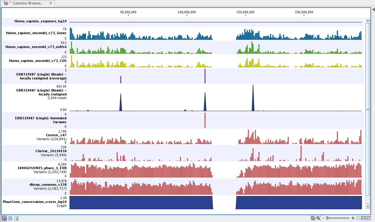
Figure 21.66: Genome Browser View to inspect identified variants in
the context of the human genome and external databases.
The Genome Browser View includes the annotated variants in context to the human reference sequence, genes, transcripts, coding regions, targeted regions, mapped sequencing reads, relevant variants in the ClinVar database as well as common variants in common dbSNP, HapMap and 1000 Genomes databases. Finally, a track with conservation scores shows the level of nucleotide conservation around each variant.
The conservation scores are based on a multiple alignment with a range of different vertebrates. The conservation in the region around each variant is particularly relevant when you consider the potential importance of the individual variants. A high conservation score could indicate that the variant is located in a region of the genome that is of great importance.
The annotated variant track can also be shown in table view. To open the table, double-click on the name of the variant track in the left side of the Genome Browser View (when opened in the View Area). The annotated variant table includes all variants and the added information/annotations (see 21.67).
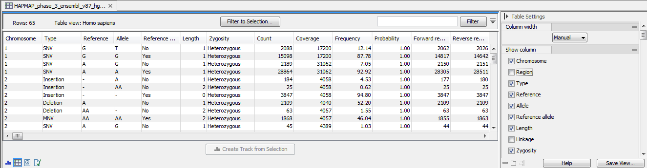
Figure 21.67: The annotated variant track opened in table view from the Genome Browser View. The table makes it easier to inspect identified variants in detail.
In figure 21.68 the annotated variant table and the Genome Browser View are shown in split view. The annotated variant table and the Genome Browser View are connected and when selecting a variant from the table by clicking on a row in the table, the Genome Browser View will automatically put the selected variant into focus. In figure 21.68 the "Zoom to base level" function (![]() ), marked with a red arrow in the lower right corner of the View Area, has been used to zoom in on the variant.
), marked with a red arrow in the lower right corner of the View Area, has been used to zoom in on the variant.
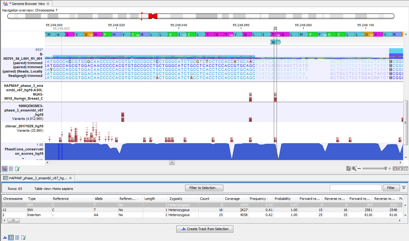
Figure 21.68: The annotated variant table and the Genome Browser View shown in split view.
The added information can support identification of candidate variants for further research. For example common genetic variants (present in the HapMap database) or variants known to play a role in drug response or other relevant phenotypes (present in the ClinVar database) can easily be singled out using the table.
Also, identified variants that are unknown in the ClinVar database can be for example prioritized based on amino acid changes. A high conservation level on the position of the variant between many vertebrates or mammals can also be a hint that this region could have an important functional role, with variants with a conservation score of more than 0.9 (PhastCons score) that should be prioritized higher. Filtering of the variants based on their annotations can be facilitated using the table filter in the top right side of the table.
Please note that in case none of the variants are present in ClinVar or dbSNP, the corresponding annotation column headers are missing from the result.