Region-level CNV track (Region CNVs)
The algorithm will produce a region-level annotation track, which contains the CNV regions detected by the algorithm. Every annotation in this track joins one or more targets from the input target track, to produce contiguous CNVs. Each CNV in the region-level tracks is characterized in terms of the following properties:
- Minimum CNV length:
- The minimum CNV length is the length of the region-level CNV annotation. This number should be interpreted as the lowest bound for the size of the CNV. The "true" CNV can extend into the adjacent genomic regions that have not be targeted.
- P-value:
- The p-value corresponds to the probability that an observation identical to the CNV, or even more of an outlier, would occur by chance under the null hypothesis. The null hypothesis is that of no CNVs in the data. The p-value for a CNV region is calculated by combining the p-values of its constituent targets (discarding any low-coverage targets) using Fisher's method.
- Fold-change (adjusted):
- The fold-change of the adjusted case coverage compared to the baseline. Negative fold-changes indicate deletions, and positive fold-changes indicate amplifications. A fold-change of 1.0 (or -1.0) represents identical coverages. The fold-changes are adjusted for statistical differences between targets with different sequencing depths. The fold-change for a CNV region is the median of the adjusted fold-changes of its constituent targets (discarding any low-coverage targets). Note: if your sample purity is less than 100%, you need to take that into account when interpreting the fold-change values. This is described in more detail in How to interpret fold-changes.
- Consequence:
- The consequence classifies statistically significant CNVs as "Gain" or "Loss".
- Number of targets:
- The total number of targets forming the (minimal) CNV region.
- Ploidy state:
- If LOH detection is enabled this column will contain the consensus ploidy state of the targets the region is composed of.
- Targets:
- A list of the names of the targets forming the (minimal) CNV region. Note however that the list is truncated to 100 characters. If you want to see all the targets that constitute the CNV region, you can use the target-level output (section 24.2.2).
- Comments:
- The comments can include useful information for interpreting individual CNV calls. The possible comments are:
- Small region: If a region only consists of 1 target, it is classified as a 'small region'. The p-value of this region is therefore based on evidence from just one target, and may be less accurate than p-values for larger regions.
- Disproportionate chromosome coverage: If a region is found on a chromosome that was determined to have disproportionate coverage, this will be noted in the comments. This means that the targets constituting this region were not used to set up the statistical models. Furthermore, the size and fold-change value of this CNV region may explain why the chromosome was detected to have disproportionate coverage.
- Low coverage: If all targets inside a region had low-coverage, then the region will be classified as a 'low-coverage' region, and will be given a p-value of 1.0. You will only see these regions in the results if you set the significance cutoff to 1.0.
Note: The region-level calls do not guarantee that a single, larger CNV will always be called in just one CNV region. This is because adjacent region-level CNV calls are not joined into a single region if their average fold-changes are sufficiently different. For example, if a 2-fold gain is detected in a region and a 3-fold gain is detected in an immediately adjacent region of equal size, then these may appear in the results as two separate CNVs, or one single CNV with a 2.5-fold gain, depending on your chosen graining level, and the fold-changes observed in the rest of the data.
How to interpret fold-changes when the sample purity is not 100%
If your sample purity is less than 100%, it is necessary to take that into account when interpreting the fold-change values.
Given a sample purity of
| fold-change in 100% pure sample |
(24.7) |
For example, if the sample purity is 40%, and you have observed an amplification with a fold-change of 3, then the fold-change in the 100% pure sample would have been:
| fold-change in 100% pure sample |
(24.8) |
For a deletion the formula for converting an observed (absolute) fold-change to the actual (absolute) fold change is:
| fold-change in 100% pure sample |
(24.9) |
For example, if the sample purity is 40%, and you have a deletion with an absolute fold-change of 1.25, then the absolute fold-change in the 100% pure sample would have been:
| fold-change in 100% pure sample |
(24.10) |
Figures 24.9 and 24.10 shows the 'true' fold changes for different observed fold-changes at different sample purities.
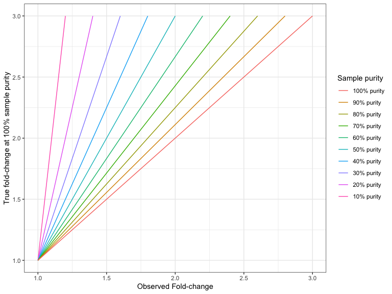
Figure 24.9: The true amplification fold-change in the 100% pure sample, for different observed fold-changes, as a function of sample purity.
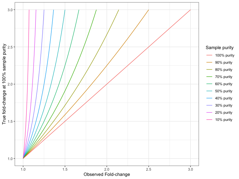
Figure 24.10: The true deletion fold-change in the 100% pure sample, for different observed fold-changes, as a function of sample purity.