- Normalization and chromosome analysis
- Prediction of target-level CNVs
- Prediction of region-level CNVs
CNV algorithm report
If you have chosen to produce an algorithm report in the output handling step of the wizard, an algorithm report will also be produced. This contains information about the statistical models of the algorithm, and can be used to evaluate how well the assumptions of the model were fulfilled. We will now present the different sections of this report.
Normalization and chromosome analysis
This section of the report is related to the first step of the CNV and LOH Detection tool, where the chromosome-level coverages are analyzed to detect any outliers. The total coverages of the case chromosomes are plotted against the total coverages of the baseline, and the detected outliers are indicated. Chromosome coverages identified as disproportionate are marked with red crosses (see figure 24.14).
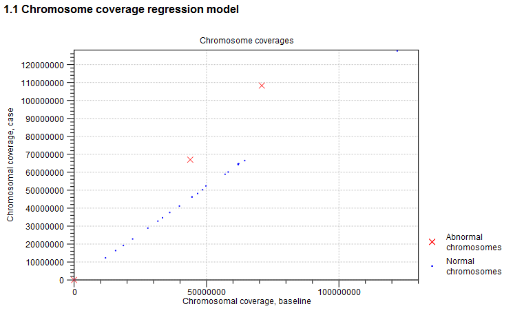
Figure 24.14: An example graph showing the coverages of the chromosomes in the case versus the baseline. In this example, three chromosomes are marked as abnormal. Two of these chromosomes are significantly amplified, and log-ratios of coverages of many targets on these chromosome are significantly higher than for targets on other chromosomes. The third outlier chromosome had zero coverage in both the case and the baseline.
The graph is followed by a table, where the detailed chromosome coverages are shown after normalization. Chromosomes with disproportionate coverage and chromosomes without any targets are marked in the 'Comment' column. These chromosomes are the ones marked with red crosses in the graph in section 1.1. of the algorithm report, and these chromosomes were not used in the coverage normalization step.
Prediction of target-level CNVs
This section of the algorithm report gives information about the statistical models used to predict target-level CNVs.Adjustment of log2-ratios The first two graphs in this section are related to the adjustment of the log-ratios of coverages as a function of log-coverage. The log-ratio of coverages for targets depends on the level of coverage of the target, as observed by Li et al. (Bioinformatics, 2012), who also proposed that a linear correction should be applied[Li et al., 2012]. In the first of the two graphs, the non-adjusted log-ratios of target coverages are plotted against the log-coverage of the targets. In the second graph, the mean log-ratios are plotted after adjustment (figure 24.15). If the model fits the data, we expect to see that the adjusted mean log-ratios are centered around 0 for all log-coverages, and the variation decreases with increasing log-coverage.
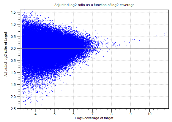
Figure 24.15: An example graph showing the mean adjusted log-ratios of coverages plotted against the log-coverages of targets, in the algorithm report of the CNV and LOH Detection tool. Here, the adjusted mean log-ratios are centered around 0.0 for most coverages, and the variation decreases with increasing log-coverage. This indicates a good fit of the model. However, at very high coverages, the adjusted log-ratios are centered higher than 0.0, which indicates that for these coverages, the model is not a perfect fit. But only very few targets are affected by this, as the points are very sparse at these high coverage levels.
Statistical model for adjusted log2-ratios In this section of the algorithm report, you can see how well the algorithm was able to model the statistical variation in the log-ratios of coverages. An example is shown in figure 24.16). A good fit of the model to the data points indicates that the variance has been modeled accurately.
To make the points more visible, double-click the figure, to open it in a separate editor. Here, you can select how to visualize the data points and the fitted model. For example, you can choose to highlight the data points in the sidepanel:
MA Plot Settings | Dot properties | Dot type | "Dot"
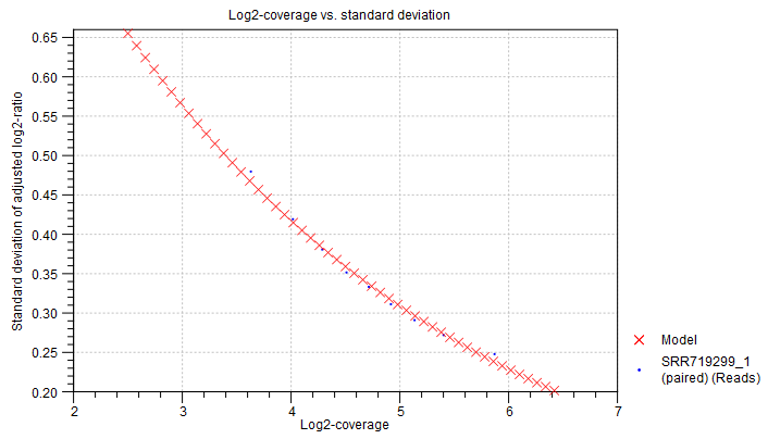
Figure 24.16: An example graph showing how the variance in the target-level mean log-ratios was modeled in the algorithm report of the Copy Number Variation Detection tool. Here, the data points are very close to the fitted model, indicating a good fit of the model to the data.
Distribution of adjusted log2-ratios in bins One of the assumptions of the statistical model used by the CNV detection tool is that the coverage log-ratios of targets are normally distributed with a mean of zero, and the variance only depends on the log-coverage of each target in the baseline. The bar charts in this section of the algorithm report show how well this assumption of the model fits the data. An example is shown in figure 24.17). A good fit of the model to the data points indicates that the variance has been modeled accurately.
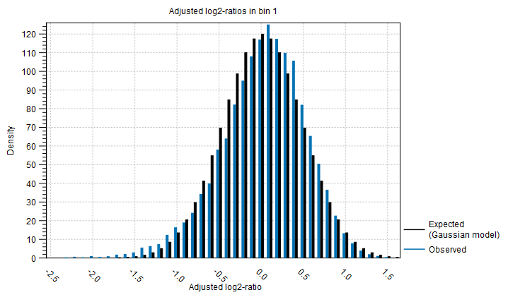
Figure 24.17: An example bar chart from the algorithm report of the Copy Number Variation Detection tool, showing how well the normal distribution assumption was fulfilled by the adjusted coverage log-ratios. Here, there is a good correspondence between the expected distribution and the observations.
Prediction of region-level CNVs
The final section of the algorithm report is related to the region-level CNV prediction. In this part of the algorithm, the chromosomes are segmented into regions of similar adjusted mean log-ratios. More segments lead to a reduced variance per segment; in the extreme, where every target forms its own segment, the variance is zero. However, more segments also mean that the model contains more free parameters, and is therefore potentially over-fitted. A value known as the Bayesian Information Criterion (BIC) gives an indication of the balance of these two effects, for any potential segmentation of a chromosome. The segmentation process aims to minimize the BIC, producing the best balance of accuracy and overfitting in the final segments.The segmentation begins by identifying a set of potential breakpoints, known as local maximizers. The number of potential breakpoints at the start of the segmentation is shown in the "# local maximizers at start" column, and the corresponding BIC score is indicated in the "Start BIC" column. Breakpoints are removed strategically one-by-one, and the BIC score is calculated after each removal. When enough breakpoints have been removed for the BIC score to reach its minimum, the final number of breakpoints is shown in the "# local maximizers at end" column, and the corresponding BIC score is indicated in the "End BIC" column. A large reduction in the number of local maximizers indicates that it was possible to join many smaller CNV regions into larger ones.
Note: The segmentation process only produces regions of similar adjusted coverage log-ratios. Each segment is tested afterwards, to identify if it represents a CNV. Therefore, the number of segments shown in this table does not correspond to the number of CNVs actually predicted by the algorithm.