Running the Empirical analysis of DGE
The Empirical Analysis of DGE tool should always be run on the original counts. This is because the algorithm assumes that the counts on which it operates are Negative Binomially distributed and implicitly normalizes and transforms these counts. If the counts have in any way been altered prior to submitting them to the Empirical Analysis of DGE tool, this assumption is likely to be compromised.
When running the Empirical analysis of DGE tool in the Genomics workbench, the user is asked to specify two parameters related to the estimation of the dispersion (Figure 27.83). Of these, the 'Total count filter cut-off' specifies which features should be considered when estimating the common dispersion component. Features for which the counts across all samples is low are likely to contribute mostly with noise to the estimation, and features with a lower cummulative count across samples than the value specified will be ignored. When the check-box 'Estimate tag-wise dispersions' is checked, the dispersion estimate for each gene will be a weighted combination of the tag-wise and common dispersion, if the check-box is un-ticked the common dispersion will be used for all genes.
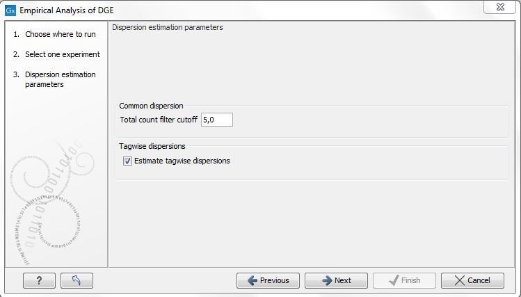
Figure 27.83: Empirical analysis of DGE: setting the parameters related to dispersion.
The Empirical analysis of DGE may be carried out between all pairs of groups (by clicking the 'All pairs' button) or for each group against a specified reference group (by clicking the 'Against reference' button), Figure 27.84. In the last case you must specify which of the groups you want to use as reference (the default is to use the group you specified as Group 1 when you set up the experiment). The user can specify if Bonferroni and FDR corrected p-values should be calculated (see Section 27.7.4).
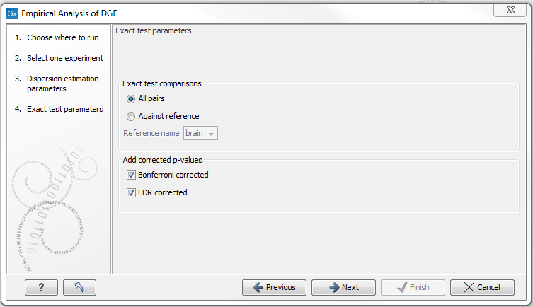
Figure 27.84: Empirical analysis of DGE: setting comparisons and corrected p-value options.
When the Empirical analysis of DGE is run three columns will be added to the experiment table for each pair of groups that are analyzed: the 'P-value', 'Fold change' and 'Weighted difference' columns. The 'P-value' holds the p-value for the Exact test. The 'Fold Change' and 'Weighted difference' columns are both calculated from the estimated 'average cpm (counts per million)' values of each of the groups. The estimated 'average cpm' values are values that are derived internally in the Exact Test algorithm. They depend on both the sizes of the samples, the magnitude of the counts and on the estimated negative binomial dispersion, so they cannot be obtained from the original counts by simple algebraic calculations. The 'Fold Change' will tell you how many times bigger the average cpm value of group 2 is relative to that of group 1. If the the average cpm value of group 2 is bigger than that of group 1 the fold change is the average cpm value of group 2 divided by that of group 1. If the average cpm value of group 2 is smaller than that of group 1 the fold change is the average cpm value of group 1 divided by that of group 2 with a negative sign. The 'weighted difference' column contains the difference between the average cpm value of group 2 and the average cpm value of group 1. In addition to the three automatically added columns, columns containing the Bonferroni and FDR corrected p-values will be added if that was specified by the user.