Calculate LOH and HRD (beta)
The Calculate LOH and HRD (beta) tool is designed to detect loss-of-heterozygosity (LOH) and Homologous recombination deficiency (HRD) from targeted research resequencing experiments.
The tool takes a target-level CNV events annotation track (from a CNV tool), somatic variants, and either germline variants or known segregating variants and optionally centromers.
To run the Calculate LOH and HRD (beta) tool, go to:
Tools | Resequencing Analysis (![]() ) | Variant Detection (
) | Variant Detection (![]() ) | Calculate LOH and HRD (beta) (
) | Calculate LOH and HRD (beta) (![]() )
)
Select the CNV target-level annotation track generated by a CNV tool and click Next.
You are now presented with choices regarding LOH detection.
- Somatic variants A track containing variants in the somatic sample. Their allele frequencies must be provided.
- Type of variant track with known variants Choose if the track with known variants is a variant database (Variant database) or a matching germline variant track (Germline variants). This will determine if LOH detection is performed in unpaired mode or in matched tumor normal mode.
- Known variants If "Variant database" is chosen above, provide a variant track of known SNPs in the population annotated with allele frequencies (e.g. dbSNP). The variant track can be restricted to the target region to improve computation time. This can be done using the Filter Based on Overlap tool, see https://resources.qiagenbioinformatics.com/manuals/clcgenomicsworkbench/current/index.php?manual=Filter_Based_on_Overlap.html. If "Germline variants" are chosen above, provide a variant track with matching germline variants. The variants are automatically filtered to heterozygous variants. For optimal performance, the variants should be high confidence.
- Normalize coverage using allele frequencies If enabled, allele frequencies will be used to find the correct coverage normalization. If a large fraction of targets are affected by say a deletion, the normalization factor used for the sample will be too low, resulting in underdetection. However, a deletion is both expected to affect the coverage and the allele frequencies and this information can be used to correct the normalization factor (see tables 25.6 and 25.7). As an example, if the control sample has copy number 2 for all targets, but the case sample has copy number 1 for all targets, the coverage after correcting for total library size should ideally be adjusted by a factor 0.5. Enabling this option is recommended for small panels where a large fraction of targets may be affected by CNV events.
- Minimum normalization, Maximum normalization If `Normalize coverage using allele frequencies` is enabled this defines the limits to the amount of normalization done.
- Minimum sample purity The lowest sample purity the model can estimate. It is hard to distinguish a sample with only a few CNV and LOH events from a sample with very low purity. Set this parameter to the lowest purity that the model is allowed to use.
- Transition factory The transition factor controls the chance of switching state. A higher transition factor makes state switches less probable.
- HMM decoding method Method for optimizing and decoding Hidden Markov Model (VITERBI or POSTERIOR).
Click Next to set the parameters related to HRD.
- Enable HRD calculation When enabled, HRD score is calculated and an HRD section is included in the report.
- Centromeres Option to define centromeres. Regions covered by provided centromeres will be excluded from the HRD calculation.
- LOH weight, LST weight, TAI weight HRD is calculated as the sum of Loss of Heterozygosity (LOH), Large-scale State Transitions (LST), and Telomeric Allelic Imbalance (TAI) scores. These three scores can be weighted by the values given here before being summed to the final HRD score.
- Minimum LOH region length (MB) Loss of Heterozygosity (LOH) regions shorter than this are ignored in the LOH score calculation. The length is given in megabases.
- Minimum LST region length (MB) Large-scale State Transitions (LST) between regions shorter than this are ignored in the LST score calculation. The length is given in megabases.
- Maximum LST region distance (MB) Large-scale State Transitions (LST) with a distance larger than this are ignored in the LST score calculation. The distance is given in megabases.
- Short LST region length (MB) Regions shorter than this are filtered out before Large-scale State Transitions (LST) score calculation. The length is given in megabases.
- Minimum merge size Remove merged regions consisting of fewer than this number of targets.
When finished with the settings, click Next to start the algorithm.
LOH detection
The algorithm implemented in the Calculate LOH and HRD (beta) tool is inspired by the following paper:
- Beroukhim et al. Inferring loss-of-heterozygosity from unpaired tumors using high-density oligonucleotide SNP arrays, PLoS Computational Biology. 2006, 2(5): 323-332 [Beroukhim et al., 2006]
Based on coverage ratios and the allele ratios of putative heterozygous germline variants the tool detects targets and regions affected by Loss-of-heterozygosity events. The tool can handle both matched tumor normal data and unpaired tumor data. In both cases variants that are assumed to be heterozygous in normal tissue has to be identified.
Tumor-normal pairs: For matched tumor normal data, a track with somatic variants and a track with germline variants will be used. The variants used to detect LOH are simply the somatic variants overlapping heterozygous germline variants.
Tumor only: For unpaired tumor data, a somatic variant track and a database of known segregating variants are used (typically dbSNP common). The variants used in LOH calculation are the somatic variants overlapping the variants in the database.
The model operates with a number of ploidy states, which are characterized by their numbers of parental and maternal alleles (Table 25.5). The state together with the tumor purity (the percentage of cells in the sample originating from the tumor) determines the expected coverage ratio and the expected allele frequencies of the heterozygous variants. As an example, if a normal diploid sample would yield 200 reads, then a sample with purity 50% and copy-number 1 (deletion) would yield 150 reads (50%*200+50%*100). That means the coverage ratio is 150/200 = 75%. Table 25.6 shows the expected coverage ratios for different states and purities.
The state together with tumor purity also determines the expected allele frequencies of heterozygous variants. As an example, consider a sample with 60% purity where the cancer cells contain a deletion in a region with two alleles, A and B. If we take 100 cells:
- 60 cells (tumor) will contain one copy of allele A
- 40 cells (normal) will contain one copy of allele A and one copy of B
The tool estimates the purity using a hidden Markov model (HMM), that is then used to predict the most probable state for each target.
|
|
|
HRD calculation
The HRD score is a count of chromosomal rearrangements that can be increased in tumors with HRD. It is calculated as the weighted sum of three different chromosomal rearrangements: The number of Telomeric Allelic Imbalances (TAI), Large-scale Transitions (LST), and long regions of Loss of Heterozygosity (LOH). The calculations are based on identified regions of copy number variations (CNV) as well as variant frequencies in a sample, which are identified beforehand.
The LOH score counts long regions with a minor allele count of zero. LOH regions spanning whole chromosomes are excluded.
The TAI score is defined as the number of regions that:
- (1) Show an imbalance from the most prevalent copy number state of the whole chromosome. Whether a telomeric region is imbalance with the rest of the chromosome, is determined by comparing the copy number state of the region nearest the telomere with the most prevalent copy number state of the whole chromosome.
- (2) Do not cross the centromere.
- (3) Extend up to the telomeres. Note, the region located closest to the end of a chromosome is considered a proxy for the telomeric region. The CNV regions underlying TAI are filtered for a minimum number of probes (merge size) and a minimum region length.
Calculation of the three scores is inspired by:
- Abkevich et al. Patterns of genomic loss of heterozygosity predict homologous recombination repair defects in epithelial ovarian cancer, British Journal of Cancer. 2012, 107(10): 1776-1782. [Abkevich et al., 2012]
- Birkbak et al. Telomeric allelic imbalance indicates defective DNA repair and sensitivity to DNA damaging agents, Cancer Discovery. 2012, 2(4): 366-375. [Birkbak et al., 2012]
- de Luca et al. Using whole-genome sequencing data to derive the homologous recombination deficiency scores. npj Breast Cancer. 2020, 6:33. [de Luca et al., 2020]
The LST score is the number of LST events. The LST score counts large rearrangements for each arm of a chromosome. The regions are merged and short regions removed iteratively. For each chromosome arm, as long as there are segments less than 3 MB, the segment at the first position, that is less than 3 MB is removed and adjacent segments across the whole chromosome arm with identical allele counts merged.
Calculate LOH and HRD algorithm report
Loss-of-heterozygosity
This section provides information related to LOH calculation. The first table shows the estimated purity and normalization factor along with confidence intervals. Low purity or a wide confidence interval for purity is an indication that the LOH predictions are uncertain. In the next table the number of targets predicted to be in each ploidy state is shown.
The next two subsections provide information useful for diagnosing potential problems with LOH detection. First, the expected coverage log-ratios for each ploidy state are shown along with the average coverage log-ratios for targets predicted to have this state. The expected coverage log-ratios are simply computed as in table 25.6 based on the estimated purity. Below the table is a plot with coverage log-ratios plotted against the base coverage. The points are colored by their predicted state and horizontal lines indicate the expected log-coverage ratio for each state (Figure 25.26).
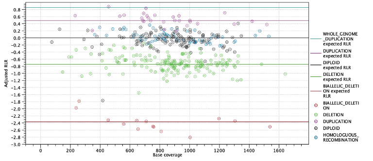
Figure 25.26: Log-coverage ratios for each target with horizontal lines indicating the expected log-coverage ratio.
Second, the expected allele frequencies for each ploidy state are shown along with the average allele frequency for variants predicted to have this state. Again the expected allele frequencies are computed as in table 25.7 based on the estimated purity. Below the table is a plot with allele frequencies plotted against their coverage. The points are colored by their predicted state and horizontal lines indicate the expected allele frequency for each state (Figure 25.27).
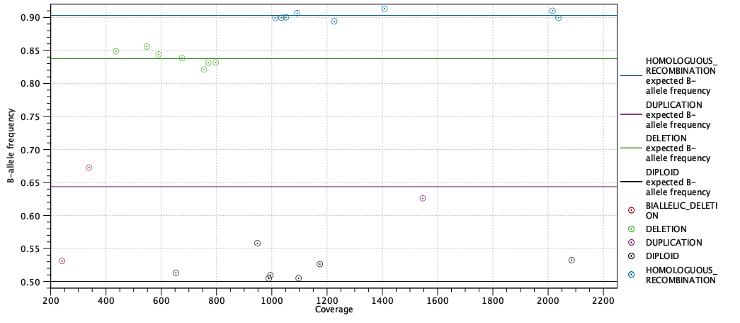
Figure 25.27: Allele frequencies for each putative heterozygous variant with horizontal lines indicating the expected allele frequencies.
HRD score
This section of the report is only included when HRD calculation is enabled in the Calculate LOH and HRD (beta) tool. The section provides a table listing the HRD score, as well as individual LOH, LST, and TAI scores. In the table is also listed the events that were counted to give the individual LOH, LST and TAI scores.
LOH regions included in the LOH score are listed in the row LOH regions. For each region, the chromosome and the start and end of the LOH region is included. As an example, the entry "2: 151M 169M" should be read as an LOH event on chromosome 2 occurring from position 51M to 169M.
Each transition included in the LST score is listed in the row LST. As an example, in the entry "S1: 1-2 0M 13M -> 1-1 13M 248M" the parts before and after the arrow describes the chromosomal states on each side of the transition and should be read as: Start of chromosome 1, minor allele count 1, major allele count 2, positions 0M-13M changes to minor allele count 1, major allele count 1, positions 13M to 248M.
For TAI, results are listed for each chromosome in the row TAI. As an example "S1 TAI 2 1-2", should be read as start of chromosome 1, TAI event, most prevalent copy number state for the whole chromosome is 2, for the TAI event minor allele count is 1 and major allele count is 2. Correspondingly, "E1 CENT 125M 248M" should be read as end of chromosome 1, region extends from end of chromosome to centromere and is not counted as TAI, positions 125M-248M and "E10 NO 2 1-1" should be read as end of chromosome 10, no TAI event, most prevalent copy number state for the whole chromosome is 2, and for the region closest to the end of the chromosome minor allele count is 1 and major allele count is 1. Hence, a TAI event is only counted when TAI is part of the annotation for a given chromosome arm.