Identify Variants (WES)
The Identify Variants (WES) workflow takes sequencing reads as input and returns identified variants as part of a Track List.
The tool runs an internal workflow, which starts with mapping the sequencing reads to the human reference sequence. Then it runs a local realignment to improve the variant detection, which is run afterwards.
Two different variant callers are used; the Low Frequency Variant Detection tool is used to call small insertions, deletions, SNVs, MNV, and replacements, and the InDel and Structural Variants tool calls larger insertions, deletions, translocations, and replacements. By the end of the variant detection, variants that have been detected by the Low Frequency Variant Detection tool with an average base quality smaller than 20 are filtered away.
In addition, a targeted region report is created to inspect the overall coverage and mapping specificity in the targeted regions.
Before starting the workflow, you will need to import in the workbench a file with the genomic regions targeted by the amplicon or hybridization kit. Such a file (a BED or GFF file) is usually available from the vendor of the enrichment kit and sequencing machine. Use the Import | Tracks tool to import it in your Navigation Area.
Run the Identify Variants (WES) workflow
To run the Identify Variants (WES) workflow, go to:
Ready-to-Use Workflows | Whole Exome Sequencing (![]() ) | Somatic Cancer (
) | Somatic Cancer (![]() ) | Identify Variants (WES) (
) | Identify Variants (WES) (![]() )
)
- Select the sequencing reads from the sample that should be analyzed (figure 17.28).
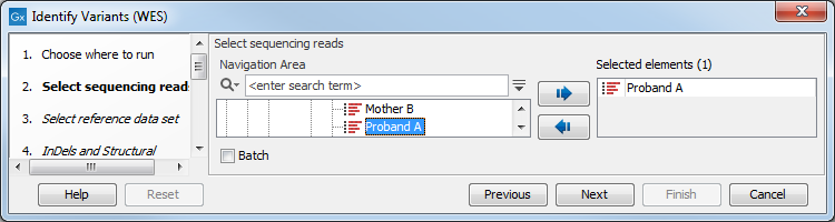
Figure 17.28: Please select all sequencing reads from the sample to be analyzed.If several samples should be analyzed, the tool has to be run in batch mode. This is done by checking "Batch" and selecting the folder that holds the data you wish to analyze.
- In the next dialog, you have to select which data set should be used to identify variants (figure 17.29).
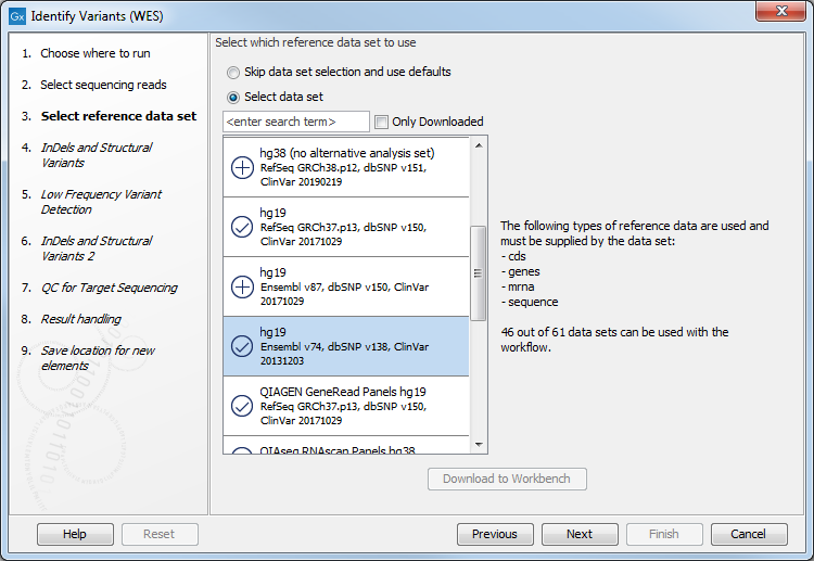
Figure 17.29: Choose the relevant reference Data Set to identify variants in your sample. - In the Indels and Structural Variants dialog you can restrict calling of such variants to the targeted regions (figure 17.30). The variants found outside the targeted region will be removed at this step in the workflow, and the output of this step twill be used as guidance in the local realignment.
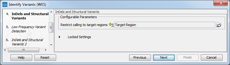
Figure 17.30: Select the track with the targeted regions from your experiment. - In the next wizard step (figure 17.31), you can specify the parameters for variant detection. You can again specify the target region track from the earlier step.
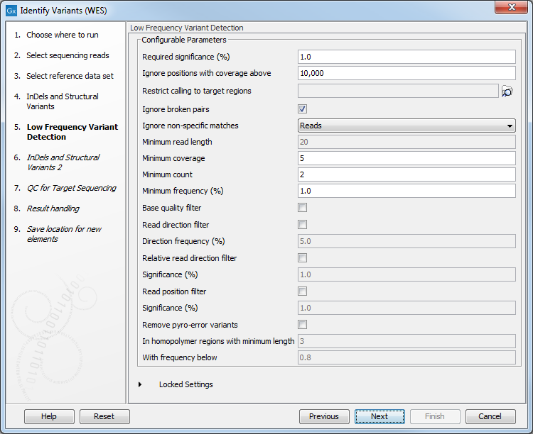
Figure 17.31: Specify the parameters for variant detection. - In the Indels and Structural Variants 2 dialog, you can can specify the same target regions track as you did earlier. This step is used to capture Indels and SNVs left after the local realignment has been performed.
- In the QC for Target Sequencing step (figure 17.32) you have to specify the track with the targeted regions from the experiment. You can also specify the minimum read coverage, which should be present in the targeted regions.
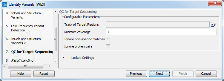
Figure 17.32: Select the track with the targeted regions from your experiment. - In the last wizard step you can check the selected settings by clicking on the button labeled Preview All Parameters.
In the Preview All Parameters wizard you can only check the settings, and if you wish to make changes you have to use the Previous button from the wizard to edit parameters in the relevant windows.
- Choose to Save your results and click Finish.
Output from the Identify Variants (WES) workflow
The Identify Variants (WES) tool produces the following outputs:
- Read Mapping (
 ) The mapped sequencing reads. The reads are shown in different colors depending on their orientation, whether they are single reads or paired reads, and whether they map unambiguously (see http://resources.qiagenbioinformatics.com/manuals/clcgenomicsworkbench/current/index.php?manual=Coloring_mapped_reads.html).
- Target Regions Coverage (
 ) The target regions coverage track shows the coverage of the targeted regions. Detailed information about coverage and read count can be found in the table format, which can be opened by pressing the table icon found in the lower left corner of the View Area.
- Target Regions Coverage Report (
 ) The report consists of a number of tables and graphs that in different ways provide information about the targeted regions.
- Structural Variants () Variant track showing the structural variants; insertions, deletions, replacements. Hold the mouse over one of the variants or right-clicking on the variant. A tooltip will appear with detailed information about the variant. The structural variants can also be viewed in table format by switching to the table view. This is done by pressing the table icon found in the lower left corner of the View Area.
- Unfiltered and Filtered Variants (
 ) Variant tracks holding the identified variants before the filters are applied (Unfiltered), and after. Filtered variants are separated into 2 tracks, one for all identified variants, and one containing larger indels. The variants can be shown in track format or in table format. When holding the mouse over the detected variants in the Track List, a tooltip appears with information about the individual variants. You will have to zoom in on the variants to be able to see the detailed tooltip.
- Track List (
 ) A collection of tracks presented together. Shows the annotated variant track together with the human reference sequence, genes, transcripts, coding regions, the mapped reads, the identified variants, and the structural variants (see figure 17.5).
It is important that you do not delete any of the produced files individually as some of the outputs are linked to other outputs. If you would like to delete the outputs, please always delete all of them at the same time.
Have first a look at the mapping report to see if the coverage is sufficient in regions of interest (e.g. > 30 ). Furthermore, check that at least 90% of reads are mapped to the human reference sequence. In case of a targeted experiment, also check that the majority of reads are mapping to the targeted region.
Afterwards please open the Track List file (see 17.33).
The Track List includes the track of identified variants in context to the human reference sequence, genes, transcripts, coding regions, targeted regions and mapped sequencing reads.
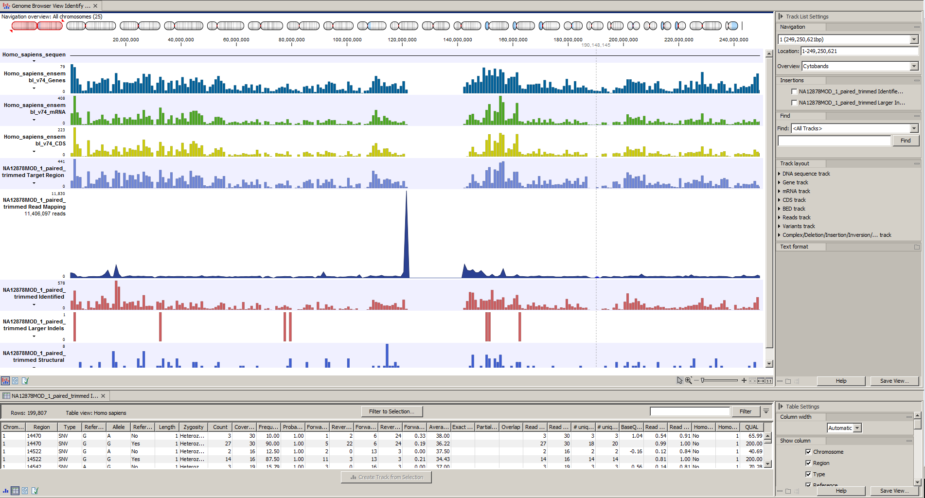
Figure 17.33: The Track List allows you to inspect the identified variants in the context of the human genome.
Open the variant track as a table to see information about all identified variants (see 17.34).
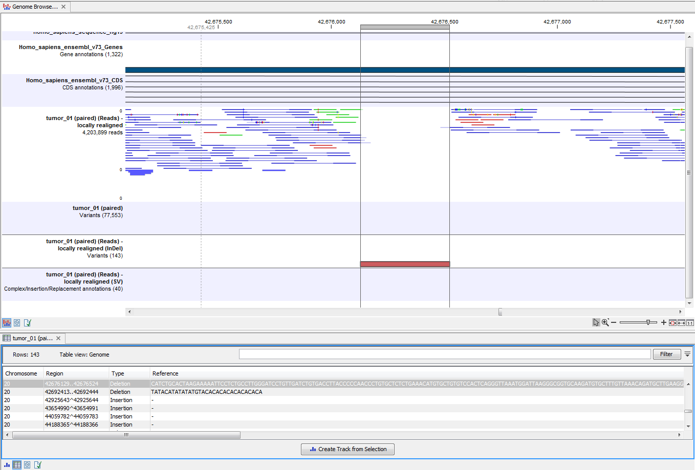
Figure 17.34: Track List with an open track table to inspect identified variants more closely in
the context of the human genome.