Beta Diversity
Beta diversity examines the change in species diversity between ecosystems.
The analysis is done in two steps. First, the tool estimates a distance between each pair of samples (see Beta diversity measures). Once the distance matrix is calculated, the beta diversity analysis tool performs Principal Coordinate Analysis (PCoA) on the distance matrices. These can be visualized by selecting the PCoA icon (![]() ) in the bottom of the Beta Diversity results (
) in the bottom of the Beta Diversity results (![]() ).
).
If you are working with an OTU table, you can specify an appropriate phylogenetic tree for computing phylogenetic diversity. In that case, you must have aligned the OTUs and constructed a phylogeny before running the Beta Diversity tool.
To run the tool, open
Microbial Genomics Module (![]() ) | Metagenomics (
) | Metagenomics (![]() ) | Abundance Analysis (
) | Abundance Analysis (![]() ) | Beta Diversity (
) | Beta Diversity (![]() )
)
Select an abundance table with more than one sample as input (i.e., an OTU table table, or a merged functional or profiling table) and set the parameters for the beta diversity analysis as shown in figure 7.4.
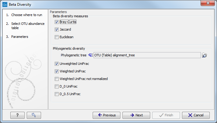
Figure 7.4:
Set up parameters for the Beta diversity tool.
The output of the tool is a 3D PCoA plot (figure 7.5) that can also be seen as a table.
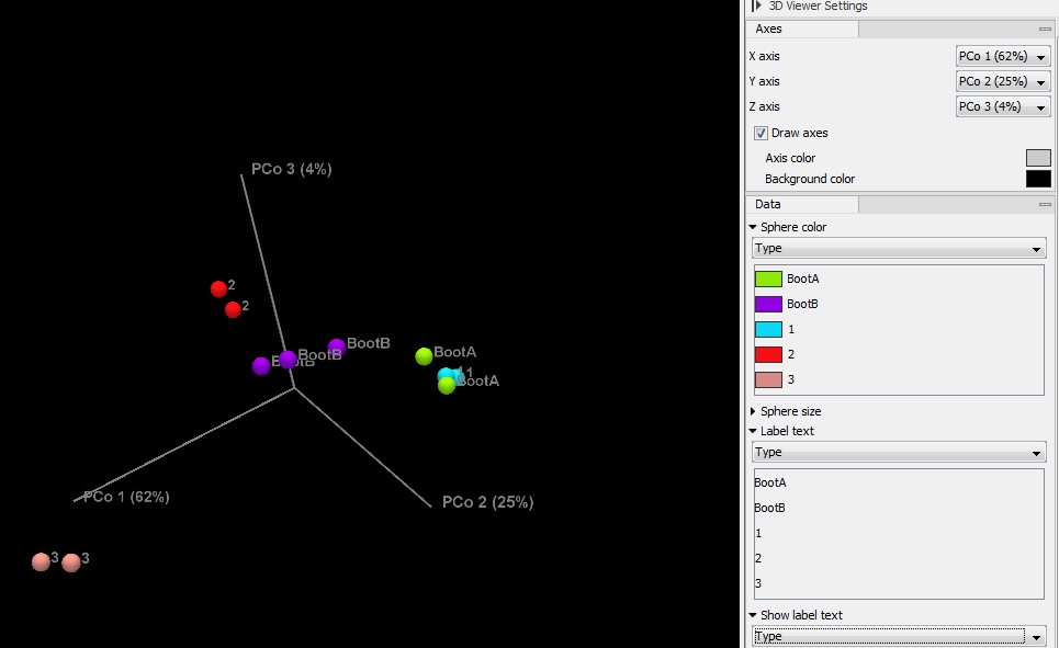
Figure 7.5:
Beta diversity results seen as a 3D PCoA.
Use the settings in the right hand side panel to explore the results and visualize them adequately.
Subsections