Compare variants in DNA and RNA
Integrated analysis of genomic and transcriptomic sequencing data is a powerful tool that can help increase our current understanding of genomic variants. The Compare variants in DNA and RNA ready-to-use workflow identifies variants in DNA and RNA and studies the relationship between the identified genomic and transcriptomic variants.
To run the ready-to-use workflow:
Toolbox | Ready-to-Use Workflows | Whole Transcriptome Sequencing (![]() ) | (Human, Mouse or Rat) | Compare variants in DNA and RNA (
) | (Human, Mouse or Rat) | Compare variants in DNA and RNA (![]() )
)
- Double-click on the Compare variants in DNA and RNA ready-to-use workflow to start the analysis. If you are connected to a server, you will first be asked where you would like to run the analysis.
- Select the RNA reads that you would like to analyze (figure 17.8). Click Next.
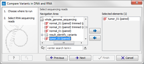
Figure 17.8: Select the RNA reads to analyze. - Select now the DNA reads to analyze (see figure 17.9). Click Next.
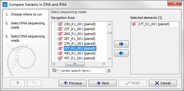
Figure 17.9: Select the DNA reads to analyze. - Configure the parameters for the RNA-Seq Analysis (figure 17.10).
If you wish to use spike-in controls, add the relevant file in the "Spike-in controls" field.
You can also specify that the reads should be mapped only in their forward or reverse orientation (it is by default set to both). Choosing to restrict mapping to one direction is typically appropriate when a strand specific protocol for read generation has been used, as it allows assignment of the reads to the right gene in cases where overlapping genes are located on different strands. Also, applying the 'strand specific' 'reverse' option in an RNA-seq run could allow the user to assess the degree of antisense transcription. Note that mate pairs are not supported when choosing the forward only or reverse only option.
Click Next.
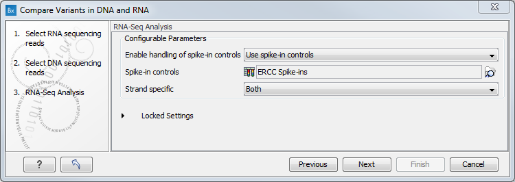
Figure 17.10: Configure the RNA-Seq Analysis. Here we specified a file for spike-in control but left the strand specific parameter to its default value. - Specify a target region for the analysis of the RNA sample with the Indels and Structural Variants tool (figure 17.11). Repeat for the DNA sample at the next step.
The targeted region file is a file that specifies which regions have been sequenced. This file is something that you must provide yourself, as this file depends on the technology used for sequencing. You can obtain the targeted regions file from the vendor of your targeted sequencing reagents. Remember that you have a hg38-specific BED file when using hg38 as reference, and hg19-specific BED file when using hg19 as reference.
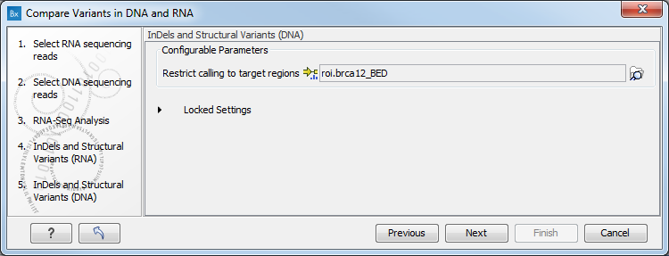
Figure 17.11: Specify the target region for the Indels and Structural Variants tool. - Set the parameters for the Low Frequency Variant Detection step for your RNA sample (see figure 17.12), and for the DNA sample at the next step. For a description of the different parameters that can be adjusted in the variant detection step, see
Low Frequency Variant Detection.
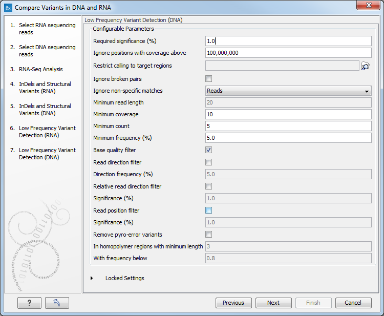
Figure 17.12: Specify the parametes for transcriptomic variant detection. - If you are working with the workflow from the Human folder, it is possible to specify in the next two steps the 1000 Genomes population that describes best your samples (see figure 17.13). Note that this step is done twice specifying the same population(s), as we annotate first the track that will contain all variants found (Union), and then the track that will contain variants that are shared between DNA and RNA (Intersection).
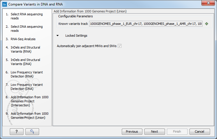
Figure 17.13: Select the relevant population from the drop-down list.Under "Locked settings" you can see that "Automatically join adjacent MNVs and SNVs" has been selected. The reason for this is that many databases do not report a succession of SNVs as one MNV as is the case for the Biomedical Genomics Workbench, and as a consequence it is not possible to directly compare variants called with Biomedical Genomics Workbench with these databases. In order to support filtering against these databases anyway, the option to Automatically join adjacent MNVs and SNVs is enabled. This means that an MNV in the experimental data will get an exact match, if a set of SNVs and MNVs in the database can be combined to provide the same allele.
Note: This assumes that SNVs and MNVs in the track of known variants represent the same allele, although there is no evidence for this in the track of known variants.
- Repeat the previous steps to specify the Hapmap population that characterizes best your samples. Note that this step is done twice specifying the same population, as we annotate first the track that will contain all variants found (Union), and then the track that will contain variants that are shared between DNA and RNA (Intersection).
- Click Next to go to the result handling step. Preview All Parameters allows you to view all parameters, but not edit them. Choose to save the results and click Finish to select a location to save the results and start the analysis.
Nine different output are generated:
- A DNA Read Mapping and a RNA Read Mapping (
 ) The mapped DNA or RNA sequencing reads. The sequencing reads are shown in different colors depending on their orientation, whether they are single reads or paired reads, and whether they map unambiguously. For the color codes please see the description
in (see Mapping view settings).
) The mapped DNA or RNA sequencing reads. The sequencing reads are shown in different colors depending on their orientation, whether they are single reads or paired reads, and whether they map unambiguously. For the color codes please see the description
in (see Mapping view settings).
- A DNA Mapping Report and a RNA Mapping Report (
 ) This report contains information about the reads, reference, transcripts, and statistics (see RNA-seq report for details).
- An RNA Gene Expression (
 ) A track showing gene expression annotations. Hold the mouse over or right-clicking on the track. If you have zoomed in to nucleotide level, a tooltip will appear with information about gene name and expression values.
- An RNA Transcript Expression () A track showing transcript expression annotations. Hold the mouse over or right-clicking on the track. A tooltip will appear with information about e.g. gene name and expression values.
- A Filtered Variant Track with All Variants Found in DNA or RNA (
 ) This track shows all variants that have been detected in either RNA, DNA or both.
- A Filtered Variant Track with Variants Found in Both DNA and RNA () This track shows only the variants that are present in both DNA and RNA. With the table icon (
 ) found in the lower left part of the View Area it is possible to switch to table view. The table view provides details about the variants such as type, zygosity, and information from a range of different databases.
- A Genome Browser View Variants Found in DNA and RNA (
 ) A collection of tracks presented together. Shows the annotated variants track together with the human reference sequence, genes, transcripts, coding regions, and variants detected in ClinVar and dbSNP (see figure 17.14).
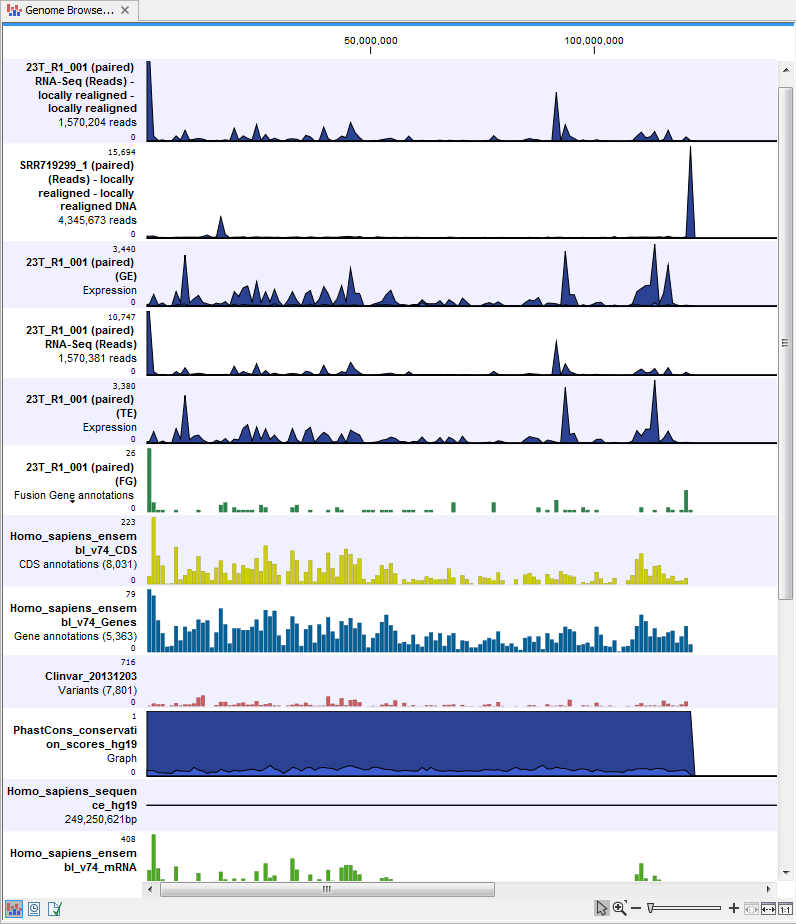
Figure 17.14: The genome browser view makes it easy to compare a range of different data.
The three most important tracks generated are the Variants found in both DNA and RNA track, All variants found in DNA or RNA track, and the Genome Browser View. The Genome Browser View makes it easy to get an overview in the context of a reference sequence, and compare variant and expression tracks with information from different databases. The two other tracks (Variants found in both DNA and RNA track and All variants found in DNA or RNA track) provides detailed information about the detected variants when opened in table view.