The docking algorithms
In the docking simulation, a number of variables defining the ligand binding mode are optimized, to achieve a good docking score. There are thus two important aspects of the docking simulation, namely the search algorithm and the docking scoring function.
The docking scoring function
A perfect search will return the binding mode with the best possible docking score. Docking results will therefore never get better than the scoring function used. As the scoring function has to be evaluated for numerous different binding modes, the complexity of the function influences greatly how much time is needed to do the docking simulation. The scoring function should therefore be as simple as possible, while still being able to distinguish between favorable and poor protein-ligand interactions. The docking score used in the Drug Discovery Workbench is the PLANTSPLP score [Korb et al., 2009]. This score has a good balance between accuracy and evaluation time. The score mimics the potential energy change, when the protein and ligand come together. This means that a very negative score corresponds to a strong binding and a less negative or even positive score corresponds to a weak or non-existing binding.
The score is listed in the Docking Results Table as "Score".
The
![]() term is a sum over contributions from all heavy atom contacts between the ligand and the molecules included in the binding site setup. It scores the complementarity between binding site and ligand by rewarding and punishing different types of heavy atom contacts (inter atom distance below ~5.5 Å).
term is a sum over contributions from all heavy atom contacts between the ligand and the molecules included in the binding site setup. It scores the complementarity between binding site and ligand by rewarding and punishing different types of heavy atom contacts (inter atom distance below ~5.5 Å).
Five different types of contacts are defined:
Rewarded contacts
- Hydrogen bond interactions
- Lone-pair - metal ion interactions
- Non-polar interactions
Punished contacts
- Non-polar - polar contacts
- Repulsive contacts:
- Hydrogen bond donor-donor contacts
- Hydrogen bond donor-metal contacts
- Hydrogen bond acceptor-acceptor contacts
These contact types are associated with a pairwise linear potential (PLP), which determines the distance-dependence of the contribution to the score. This is shown in figure 9.58.
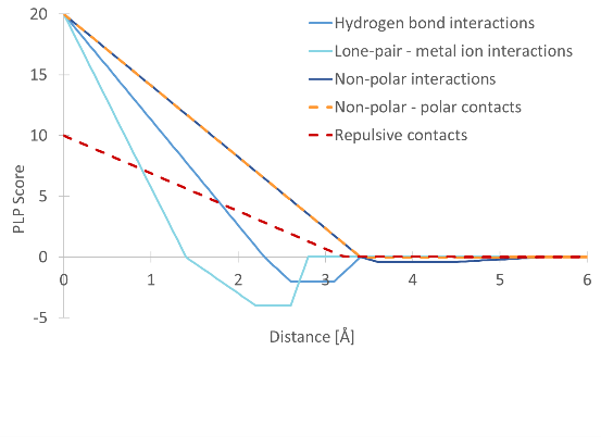
Figure 9.58: The pairwise linear potentials defining the score contributions for different types of heavy atom contacts.
Some of these contributions to the score can be displayed in the Docking Results Table. They are accessible from the 'Show column' category in the Side Panel. The contribution from hydrogen bond interactions is listed as 'Hydrogen bond score'. The contribution from lone-pair - metal ion interactions is listed as 'Metal interaction score'. The non-polar interactions, non-polar - polar contacts, and the repulsive contacts are combined in the 'Steric interaction score' contribution.
The
![]() term punishes internal heavy atom clashes in the ligand and strain resulting from unfavorable bond rotations. This contribution to the score is also accessible from the table Side Panel, and is listed as 'Ligand conformation penalty'.
term punishes internal heavy atom clashes in the ligand and strain resulting from unfavorable bond rotations. This contribution to the score is also accessible from the table Side Panel, and is listed as 'Ligand conformation penalty'.
As the score is a sum over contributions, a large ligand can get a better score than a small one, simply due to its size. When comparing scores for different molecules, this effect has to be considered and kept in mind.
The search algorithm
In a docking simulation, the variables to optimize are those that define a binding mode. Namely, the rotation angle for all rotatable (flexible) bonds in the ligand (figure 9.59), the position of the ligand within the binding site (translation), and the overall rotation of the ligand with respect to the protein. It is not feasible to do an exhaustive search with this number of variables.
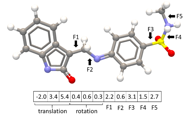
Figure 9.59: Variables defining a binding mode.
It is the docking scoring function, described above, that should be minimized with respect to the variables. The minimization problem can be envisioned as a landscape with hills and valleys, and the job is to find the deepest valley while being blindfolded, and without having to visit every point on the landscape. If there were only two variables to optimize, it would be like a familiar landscape with a latitude and a longitude to specify a point. When there are more variables, as in the case of a binding mode, the landscape is much more complex to search, with many hills and valleys in many dimensions. Fortunately, the same methods can be used as when searching for a minimum in two dimensions. The problem can be divided in two; finding a point close to the deepest valley (global optimization problem) and finding the deepest point in a valley close-by (local optimization problem).
In the docking simulation, the global search space is sampled in a number of iterations, combined with local optimizations. The number of sample iterations can be adjusted in the Dock Ligands and Screen Ligands wizards (Number of iterations for each ligand). Each iteration is independent of the others, and below is described the operations carried out for each sample iteration.
A sample iteration: A population of 20 potential binding modes is generated, by assignment of random values to the variables defining a binding mode. If binding pockets are included in the Binding Site Setup (Setup Binding Site), the binding modes are required to have at least one heavy atom inside a pocket. A binding mode initially positioned outside the binding pockets is therefore translated so as to fulfil this requirement. For each of the 20 binding modes, a local optimization with respect to the docking score is carried out, using the simplex method for function minimization [Nelder and Mead, 1965] (the simplex method is described in detail below). This is a search for the deepest point in a valley close to the initial random position. The best scoring of the 20 resulting binding modes is selected for a more refined simplex minimization. Finally, this optimized binding mode is returned from the iteration. The binding mode returned from the iteration is compared to the best scoring binding mode found so far in all iterations. If the new found binding mode has an even better score, it is saved, otherwise it is discarded. Now a new iteration can start. Each sample iteration starts from a random point in the search space. The overall search is therefore stochastic in nature, and the final result will not be exactly the same between executions, even when the same input and settings are used. However, if the results are not highly similar, it is a sign that the sampling is not sufficient (increase the 'Number of iterations for each ligand' parameter), or that a number of binding modes are equally valid.
As the iterations are independent, the overall number of iterations can be split in several 'runs', each taking their share of the iterations. This is done automatically to exploit all available CPU cores. If 'Number of docking results returned for each ligand' is set to more than one in the Dock Ligands or Screen Ligands wizards, the docking simulation is divided in at least this number of runs, and the best scoring binding modes from each of these runs are kept and returned, instead of only returning the overall best scoring binding mode.
Simplex method for function minimization: The simplex search starts from the point specified by random values [i, j, ...] assigned to the variables. To initialize the simplex minimization, N new binding modes should be generated (where N is the number of variables, see figure 9.59). These binding modes should not be too different from the input binding mode, so they are generated by shifting each variable in the initial binding mode with a small offset, ![]() :
:
For all N + 1 binding modes (points in the search space), the docking score (the function value) is evaluated.
The example below illustrates the fundamental steps in the search process. The example only has two variables (N = 2), and the color scale indicates the function values (the score, in our case). Hilltops are dark blue and valleys are dark red.
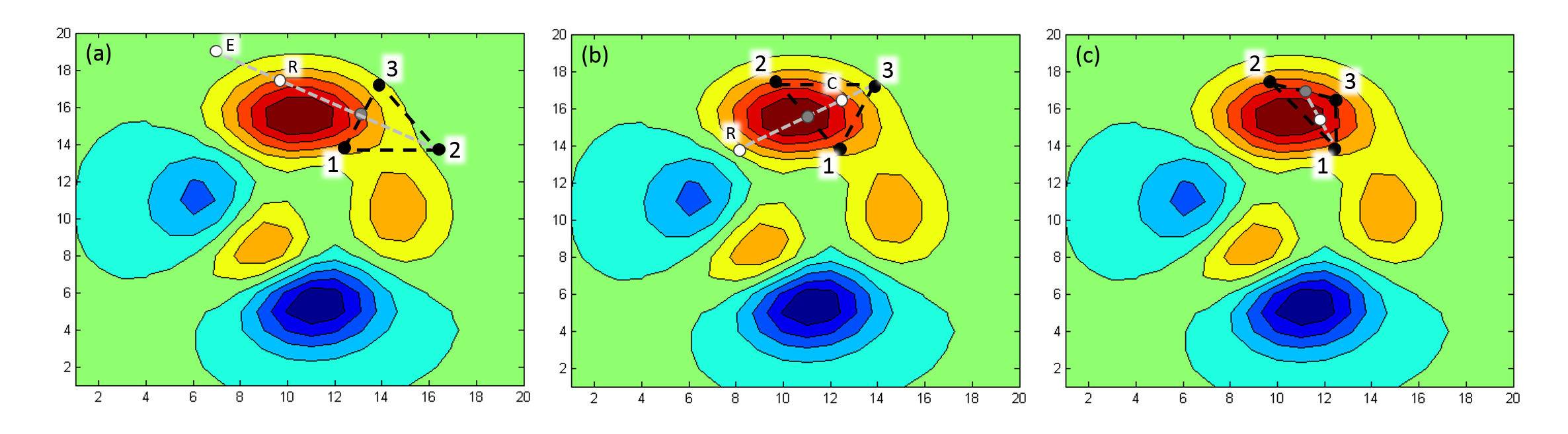
Figure 9.60: Schematic of steps taken in a Simplex local optimization.
In (a), the initial three (N + 1) points have been evaluated.
For each step in the simplex minimization, the point with the highest function value is moved to a new position.
To find the new position, the point with the highest function value is reflected in the centroid formed by all the other N points. The centroid is the mean position of the N points, in all of the coordinate directions. In a two dimensional search, the centroid is therefore the point on the line, midway between the two best scoring points (the gray points in figure 9.60). In (a), point 2 has the highest function value, and is reflected through the centroid to the white point marked "R". The function is evaluated at this point, and if it is lower than the original point, the step is taken. However, if the value is lower than for all the other points, as in this case, it could be a sign that the step was straight downhill. The reflection is therefore "extended", so as to take a larger step.
In (a), the extended point is white and marked with an "E". The function is evaluated in the extended point, and if this point is better than the reflected point, the extended step is taken instead. In figure 9.60, the extended point is worse than the reflected, and therefore the reflected point is kept.
In (b), point 2 has moved to its new position, and the point with the highest function value is now 3. When 3 is reflected in the centroid between the other points to the white point marked "R", the function value is slightly higher than in the original point. The reflected step is therefore not taken. Instead, a "contracted" step is taken, shown in (b) as a white point marked "C". The contracted point is on the reflection line, but halfway between the centroid point and the original point.
In (c), point 3 has moved to its new position, and the point with the highest function value is now 1. The reflected point is not indicated on the figure, but it is clearly uphill from the other points, and is therefore rejected. Instead, the contracted step is taken, indicated as the white point.
In this way, the search continues until the difference between the highest and lowest docking scores (for the N + 1 points), divided by the size of the lowest score, is below 0.01 (convergence), or until 2000 steps have been taken.
The refined simplex minimization, carried out for the best scoring binding mode of the 20 in the iteration population, is different from the process described above in two ways: 1) The initial point is not based on random values, it is instead the optimized binding mode returned from the initial simplex minimization. 2) The search is continued until the difference between the highest and lowest scores (for the N + 1 points), divided by the size of the lowest score, is below 0.0001, or until 2000 steps have been taken.