The Genome Browser
The Genome Browser view is a collection of tracks. Each track in a Genome Browser view is tied to the same underlying genomic co-ordinate set, making visualization and comparison of different results and data types simple and intuitive.Annotations and variant information are provided together with the human reference genome via our Data Management. Datasets, e.g. in GFF of VCF format, from resources not provided for download by Biomedical Genomics Workbench can be imported into the Navigation Area using the import option found in the toolbar:
Toolbar | Import (![]() ) | Tracks
) | Tracks
To illustrate this a Genome Browser view is shown in figure 2.8 to figure 2.13. It consists of the following tracks, all tied to the human hg19 reference: genomic sequence, gene, coding sequence (CDS), a read mapping, and variants. In figure 2.8 we have used the zoom tools to zoom all the way in on a SNV that is found in a coding region.
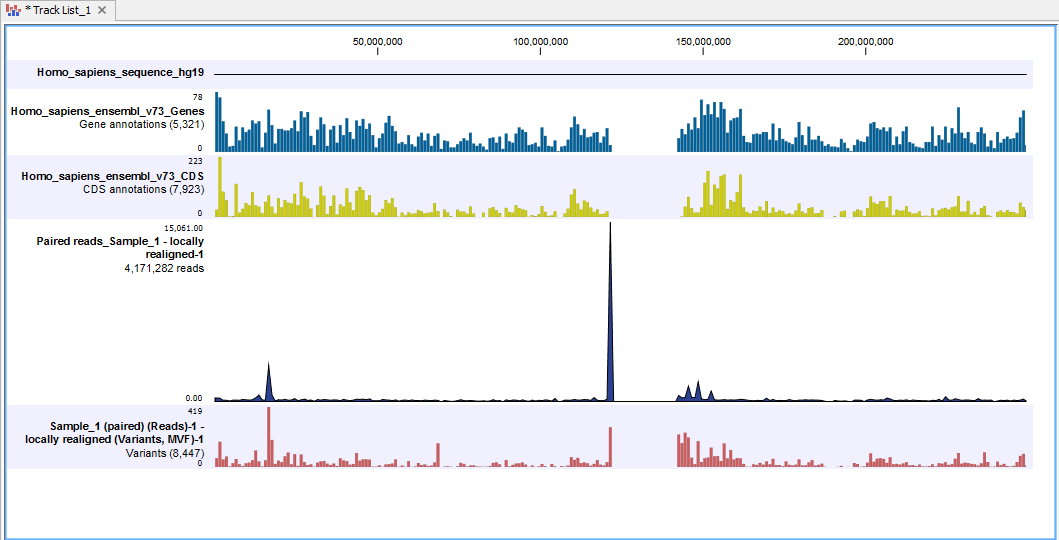
Figure 2.8: A Genome Browser view with a genomic sequence track, a gene track, a coding sequence (CDS) track, a read mapping track, and a variant track.
A Genome Browser view like the one shown in figure 2.8, allows for a complete overview of reads mapped to a reference and identified variants. You can see how many reads and variants you have, and you can compare them to the complete human genome, genes and coding regions.
How to zoom in a Genome Browser view
One way to zoom in to take a closer look at the reads and variants is to use the zoom tools. These are located in the lower right corner of the view area (see figure 2.9). Click and hold down the mouse button for a second or two on the relevant icon. This can be either an arrow or a magnifying glass. By clicking the magnifying glass icon, three icons will appear. These can be used for zooming in, zooming out, or panning. The different zoom options are described in detail in the Biomedical Genomics Workbench reference manual in the section entitled "Zoom and selection in View Area".
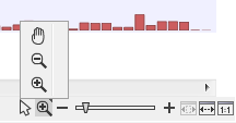
Figure 2.9: Click and hold down the mouse button for a second or two on the mangnifying glass icon until additional icons appear. Select the arrow to activate the "selection" tool. This can be used to select user-defined regions.
An quick and easy way to zoom in on a particular region is to first use the selection tool, which is activated by clicking on the arrow shown in figure 2.9). You can then select specific regions by clicking on the relevant point in the track and, keeping the mouse button depressed, dragging across the area that you wish to zoom in on. This selects the region. Once selected, you can use the "Zoom to selection" tool (shown in figure 2.10) to zoom in on the selected region.
It is also possible to zoom in just using the mouse: hold down the "Alt" key while scrolling with the mouse wheel. This zooms in (or out) on the region that is in focus in the View Area.
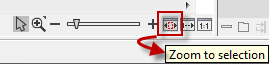
Figure 2.10: The "Zoom to selection" tool can be used to zoom in on a selected region. Next to the "Zoom to selection" icon you can find the "Zoom to fit" icon that can be used to zoom all the way out. The "Zoom slider" on the left side of the "Zoom to selection" can also be used to zoom in and out.
When clicking on the "Zoom to selection" icon, you will zoom in on the region that you have selected, and you will be able to see more and more details as you zoom in. This is shown in figure 2.11 and figure 2.12.
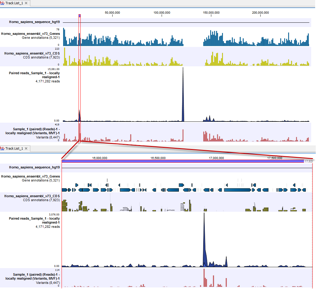
Figure 2.11: When zooming in on a selected region more and more details become visible. In this image, the individual genes are visible. To distinguish the individual exons, you would have to zoom in a bit further.
In figure 2.12 the presence of SNVs can be seen in the variant track and an overview of the mapping at that region in the mapping can be focused on.
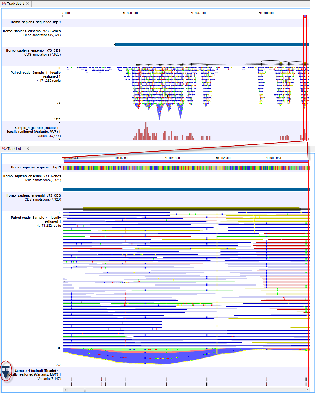
Figure 2.12: Zooming in reveals more details in all tracks.
To expand the depth of the reads track to view more details of the reads in a specific region, simply place the mouse cursor near the bottom of the left side of the genome Browser view, where the track names are, hold down the mouse and drag downwards. This is illustrated in the lower left side of figure 2.12. Here, the blue line with the arrow under it (within a red circle) illustrates where you would place the mouse cursor to be able to expand the depth of the track. In this figure, the four bases in the genomic reference sequence can be discerned via the color coding. The color codes for each of the bases are: A=red, C=blue, G=yellow, and T=green. Particular SNVs can also be discerned at this zoom level. The color of the reads indicates whether a read is part of an intact pair (blue), is a single read or a member of a broken pair mapped in the forward direction relative to the reference (green), or a single read or a member of a broken pair mapped in the reverse direction relative to the reference (red). Reads that could map equally well to other locations in the reference are colored yellow.
Figure 2.13 shows the view after zooming in on one specific SNV. By looking at the other tracks at that point, we can see that this SNV is found in a gene. The tooltip, which comes up with the mouse cursor hovers over the SNV in the variant track reveals that this is a heterozygous mutation occurring in 29 out of 447 reads. Full details about the variants in a track are shown in the table view of the track, as described in the next section.
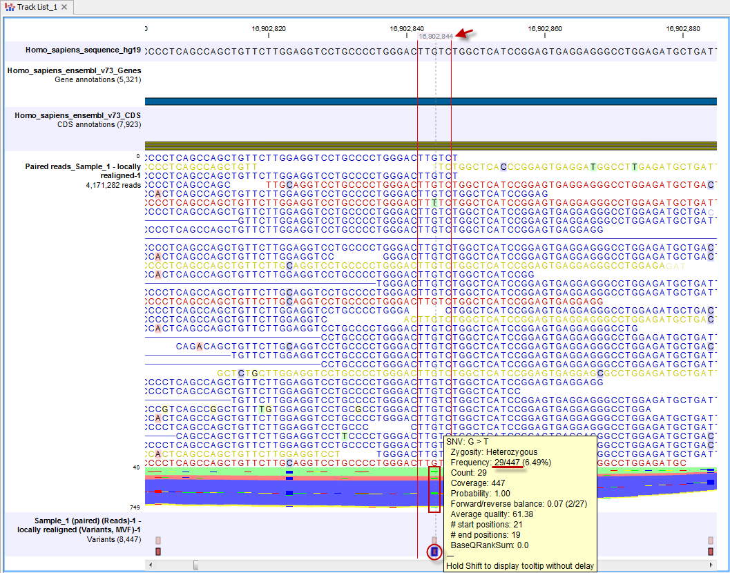
Figure 2.13: We have now zoomed in on one specific SNV that is found in a coding region. By holding the mouse over the variant, a tooltip will appear that provide further information about the specific variant. In this case we have found a heterozygous SNV. The normal base at this position is G but in some of the reads you will see a "T". Actually you can only see one "T" in the reads, but if you look in the stacked reads, which are those in the color mass where you cannot see each individual read represented, there are four green lines (read box) indicating that there are Ts at this position in more reads. When holding the mouse over an individual SNV, as highlighted in the red circle, a tooltip will appear with information about the SNV. This tooltip informs us that 29 Ts are observed in the 447 reads covering this particular position. When hovering the mouse cursor over a particular base in the reference track, the genomic position for this base is shown, as highlighted with a red arrow here.
How to open a table in split view The table view of a track provides the details of the information that is presented in the track itself. It is often useful to view the table at the same time as the track, this is done by opening the table in a split view.
From an individual track open in the Viewing area of the Workbench, this can be done by depressing the Ctrl key and clicking using the mouse on the small icon of a table at the bottom of the view.
From a genome Browser view open in the Viewing area, the table view of a particular track can be opened in a split view by double-clicking on the track name in the list. This is shown in figure 2.14.
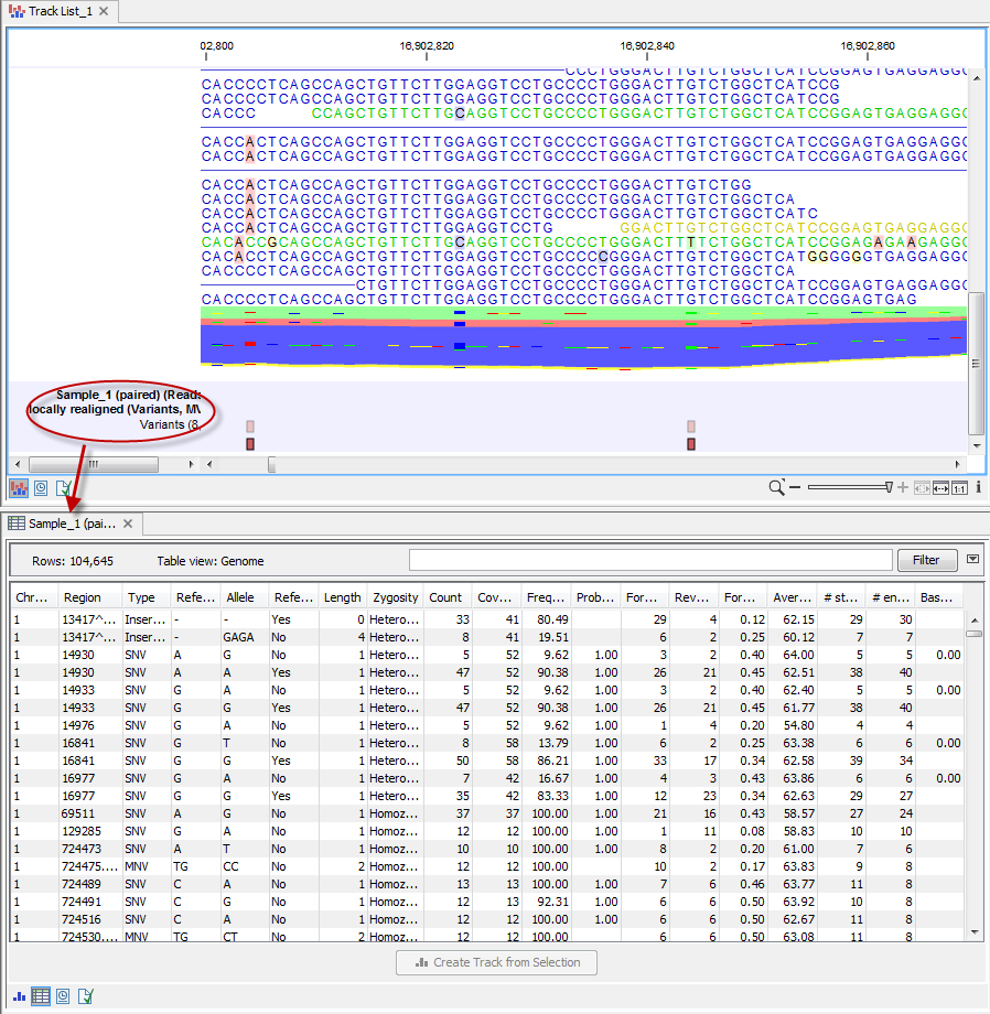
Figure 2.14: Double-click on the track name in the left side of the view area to open the table view shown in split view. When opening a track directly from the genome browser view, the table and track are linked. Hence, when selecting a row in the table by clicking on this row, this specific position in the track will be brought into focus.
The table and the track are linked, which means that clicking on a particular row in the table brings that position into focus in the Genome Browser view. For example, if you wished to jump to a particular SNV in the Genome Browser view, you could click on the row in the variant track table. This is shown in figure 2.15.
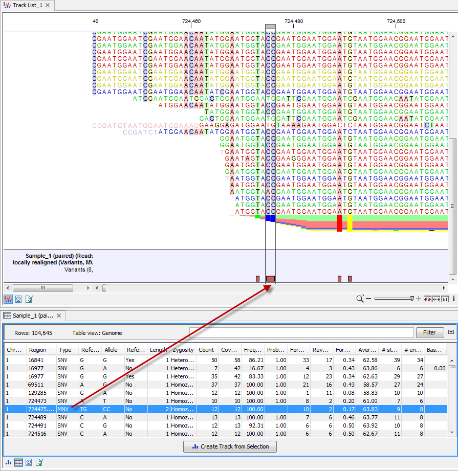
Figure 2.15: When you click on an entry in the table this position will automatically be brought into focus. Here, a row with information about an MNV, which is variant consisting of two or more SNVs, was clicked on. This brought the location of that MNV into focus in the graphical view. To jump directly to a detailed view of a position, zoom the graphical view to the desired level first and then click on the row in the table view.
Add tracks to a Genome Browser view
The most simple way to add a track to the Genome Browser view is simply to locate the file in the Navigation Area, click on the file while holding down the mouse key and drag it into the genome Browser view in the View Area. When you drop the file in the Genome Browser view, the track will be added to the Genome Browser view (figure 2.16).
Note! After having added a new track to the Genome Browser view, an asterisk has appeared on the Genome Browser view tab. This indicates that the Genome Browser view must be saved if you wish to keep the track that has been added.
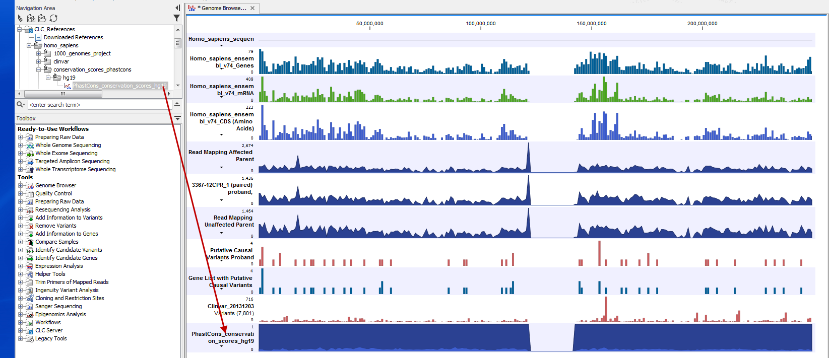
Figure 2.16: The conservation score track has been added to the Genome Browser view by dragging the track from the Navigation Area into the Genome Browser view in the View Area.