CNV and LOH Detection
The CNV and LOH Detection tool is designed to detect copy number variations (CNVs) and loss-of-heterozygosity (LOH) from targeted resequencing experiments.
The tool takes read mappings, target regions and optionally variant tracks as input, and produces amplification and deletion annotations. The annotations are generated by a 'depth-of-coverage' method, where the target-level coverages of the case and the controls are compared in a statistical framework using a model based on 'selected' targets. Note that to be 'selected', a target has to have a coverage higher than the specified coverage cutoff AND must be found on a chromosome that was not identified as a coverage outlier in the chromosomal analysis step. If fewer than 50 'selected' targets are found suitable for setting up the statistical models, the CNV tool will terminate prematurely. If a somatic variant track is provided the tool can use B allele frequencies to improve the normalization of target coverages in small panels and to infer LOH.
The algorithm implemented in the CNV and LOH Detection tool is inspired by the following papers:
- Li et al., CONTRA: copy number analysis for targeted resequencing, Bioinformatics. 2012, 28(10): 1307-1313[Li et al., 2012].
- Niu and Zhang, The screening and ranking algorithm to detect DNA copy number variations, Ann Appl Stat. 2012, 6(3): 1306-1326 [Niu and Zhang, 2012].
- Beroukhim et al. Inferring loss-of-heterozygosity from unpaired tumors using high-density oligonucleotide SNP arrays, PLoS Computational Biology. 2006, 2(5): 323-332 [Beroukhim et al., 2006]
For more information, you can also read our whitepaper: https://digitalinsights.qiagen.com/files/whitepapers/Biomedical_Genomics_Workbench_CNV_White_Paper.pdf.
The CNV and LOH Detection tool identifies CNV regions where the normalized coverage is statistically significantly different from the controls.
The algorithm carries out the analysis in several steps.
- Base-level coverages are analyzed for all samples, and a robust coverage baseline is generated using the control samples.
- Chromosome-level coverage analysis is carried out on the case sample, and any chromosomes with unexpectedly high or low coverages are identified.
- Sample coverages are normalized, and a global, target-level statistical model is set up for the variation in fold-change as a function of coverage in the baseline.
- Each chromosome is segmented into regions of similar fold-changes.
- The expected fold-change variation in region is determined using the statistical model for target-level coverages. Region-level CNVs are identified as the regions with fold-changes significantly different from 1.0.
- If chosen in the parameter steps, gene-level CNV calls are also produced.
Based on coverage ratios and the allele ratios of putative heterozygous germline variants the tool can also detect targets and regions affected by Loss-of-heterozygosity events. The tool can handle both matched tumor normal data and unpaired tumor data. In both cases variants that are assumed to be heterozygous in normal tissue has to be identified.
Tumor-normal pairs: For matched tumor normal data, a track with somatic variants and a track with germline variants will be used. The variants used to detect LOH are simply the somatic variants overlapping heterozygous germline variants.
Tumor only: For unpaired tumor data, a somatic variant track and a database of known segregating variants are used (typically dbSNP common). The variants used in LOH detection are the somatic variants overlapping the variants in the database.
The model operates with a number of ploidy states, which are characterized by their numbers of parental and maternal alleles (Table 24.1). The state together with the tumor purity (the percentage of cells in the sample originating from the tumor) determines the expected coverage ratio and the expected allele frequencies of the heterozygous variants. As an example, if a normal diploid sample would yield 200 reads, then a sample with purity 50% and copy-number 1 (deletion) would yield 150 reads (50%*200+50%*100). That means the coverage ratio is 150/200 = 75%. Table 24.2 shows the expected coverage ratios for different states and purities.
The state together with tumor purity also determines the expected allele frequencies of heterozygous variants. As an example, consider a sample with 60% purity where the cancer cells contain a deletion in a region with two alleles, A and B. If we take 100 cells:
- 60 cells (tumor) will contain one copy of allele A
- 40 cells (normal) will contain one copy of allele A and one copy of B
The tool estimates the purity using a hidden Markov model (HMM), that is then used to predict the most probable state for each target.
|
|
|
Running the CNV and LOH Detection tool
To run the CNV and LOH Detection tool, go to:
Toolbox | Resequencing Analysis (![]() ) | CNV and LOH Detection (
) | CNV and LOH Detection (![]() )
)
Select the case read mapping and click Next.
You are now presented with choices regarding the data to use in the CNV prediction method, as shown in figure 24.4.
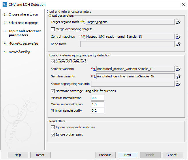
Figure 24.4: The first step of the CNV and LOH detection tool.
- Target regions track An annotation track containing the regions targeted in the experiment must be chosen. This track must not contain overlapping regions, or regions made up of several intervals, because the algorithm is designed to operate on simple genomic regions.
- Merge overlapping targets When enabled, overlapping target regions will be merged into one larger target region by expanding the first region to include all the bases of the overlapping targets, regardless of their strandedness. CNV calls are made on this larger region of merged amplicons, considered to be of undefined strand if it originated from both + and - stranded targets.
- Control mappings You must specify at least one read mapping or coverage table. The control mappings will be used to create a baseline by the algorithm. Coverage tables can be generated using the the QC for Targeted Sequencing tool, see . When using coverage tables it is important to use the same target region and settings for handling non-specific matches and broken pairs in this tool and in QC for Targeted Sequencing. For the best results, the controls should be matched with respect to the most important experimental parameters, such as gender and technology. If using non-matched controls, the CNVs reported by the algorithm may be less accurate.
- Gene track Optional: If you wish, you can provide a gene track, which will be used to produce gene-level output as well as CNV-level output.
- Enable LOH detection If you enable LOH detection, the tool will predict targets and regions affected by Loss-of-heterozygosity
- Somatic variants When LOH detection is enabled a track containing variants in the somatic sample and their allele frequencies must be provided.
- Germline variants Provide a variant track with germline variants, if running the LOH detection in matched tumor normal mode. The variants are automatically filtered to heterozygous variants. For optimal performance, the variants should be high confidence.
- Known segregating variants Provide a variant track of known SNPs in the population annotated with allele frequencies (e.g. dbSNP), if running the LOH detection in unpaired mode. The variant track should be restricted to the target region. This can be done using the Filter Based on Overlap tool, see .
- Normalize coverage using allele frequencies If enabled allele frequencies will be used to find the correct coverage normalization. If a large fraction of targets are affected by say a deletion, the normalization factor used for the sample will be too low, resulting in underdetection. However, a deletion is both expected to affect the coverage and the allele frequencies and this information can be used to correct the normalization factor (see tables 24.2 and 24.3). As an example, if the control sample has copy number 2 for all targets, but the case sample has copy number 1 for all targets, the coverage after correcting for total library size should ideally be adjusted by a factor 0.5. Enabling this option is recommended for small panels where a large fraction of targets may be affected by CNV events.
- Minimum normalization, Maximum normalization If `Normalize coverage using allele frequencies` is enabled this defines the limits to the amount of normalization done.
- Minimum sample purity The lowest sample purity the model can estimate. It is hard to distinguish a sample with only a few CNV and LOH events from a sample with very low purity. Set this parameter to the lowest purity that the model is allowed to use.
- Ignore non-specific matches If checked, the algorithm will ignore any non-specifically mapped reads when counting the coverage in the targeted positions. Note: If you are interested in predicting CNVs in repetitive regions, this box should be unchecked.
- Ignore broken pairs If checked, the algorithm will ignore any broken paired reads when counting the coverage in the targeted positions.
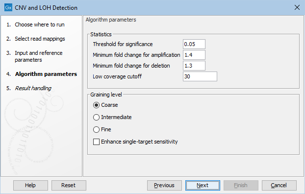
Figure 24.5: The second step of the CNV detection tool
Click Next to set the parameters related to the target-level and region-level CNV detection, as shown in as shown in figure 24.5.
- Threshold for significance P-values lower than the threshold for significance will be considered "significant". The higher you set this value, the more CNVs will be predicted.
- Minimum fold change for amplification and Minimum fold change for deletion You must specify the minimum fold changes for a CNV call for amplification and deletion.
If the absolute value of the fold change of a CNV is less than the value specified in this parameter, then the CNV will be filtered from the results, even if it is otherwise statistically significant.
For example, if a minimum fold-change of 1.5 is chosen for amplification, then the adjusted coverage of the CNV in the case sample must be 1.5 times higher than the coveage in the baseline for it to pass the filtering step.
Similarly, if a minimum fold-change of 1.5 is chosen for deletion, then the adjusted coverage of the CNV in the case sample must be 1.5 times lower than the coverage in the baseline.
If you do not want to filter on the fold-change, enter 0.0 in these fields. Also, if your sample purity is less than 100%, it is necessary to take that into account when you adjust the fold-change cutoff. This is described in more detail in How to set the fold-change cutoff when the sample purity is not 100%. Note: this value is used to filter the Region-level CNV track. The Target-level CNV track will always include full information for all targets.
- Low coverage cutoff If the average coverage of a target is below this value, it will be considered "low coverage" and it will not be used to set up the statistical models, and p-values will not be calculated for it in the target-level CNV prediction.
- Graining level The graining level is used for the region-level CNV prediction. Coarser graining levels produce longer CNV calls and less noise, and the algorithm will run faster. However, smaller CNVs consisting of only a few targets may be missed at a coarser graining level.
- Coarse: prefers CNVs consisting of many targets. The algorithm is most sensitive to CNVs spanning over 10 targets. This is the recommended setting if you expect large-scale deletions or insertions, and want a minimal false positive rate.
- Intermediate: prefers CNVs consisting of an intermediate number of targets. The algorithm is most sensitive to CNVs spanning 5 or more targets. This is the recommended setting if you expect CNVs of intermediate size.
- Fine: prefers CNVs consisting of fewer targets. The algorithm is most sensitive to CNVs spanning 3 or more targets. This is the recommended setting if you want to detect CNVs that span just a few targets, but the false positive rate may be increased.
- Enhance single-target sensitivity All of the graining levels assume that a CNV spans more than one target. If you are also interested in very small CNVs that affect down to a single target in your data, check the 'Enhance single-target sensitivity' box. This will increase the sensitivity of detection of very small CNVs, and has the greatest effect in the case of the coarser graining levels. Note however that these small CNV calls are much more likely to be false positives. If this box is unchecked, only larger CNVs supported by several targets will be reported, and the false positive rate will be lower.
Clicking Next, you are presented with options about the results (see figure 24.6). In this step, you can choose to create an algorithm report by checking the Create algorithm report box. Furthermore, you can choose to output results for every target in your input, by checking the Create target-level CNV track box.
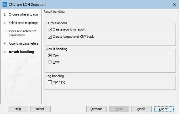
Figure 24.6: Specifying whether an algorithm report and a target-level CNV track should be created.
When finished with the settings, click Next to start the algorithm.
Copy number and fold change
When configuring the minimum fold change thresholds for calling CNVs, it can be useful to understand the difference between copy number and fold change and the relationship between tumor fold change, sample fold change and sample purity.
The copy number (CN) gives the number of copies of a gene. For a normal diploid sample the copy number, or ploidy, of a gene is 2.
The fold change is a measure of how much the copy number of a case sample differs from that of a normal sample. When the copy number for both the case sample and the normal sample is 2, this corresponds to a fold change of 1 (or -1).
The sample fold change can be calculated from the normal copy number and sample copy number. The formula differs for amplifications and deletions:
| Fold change, amplifications (CN(sample) > CN(normal)) |
(24.1) |
| Fold change, deletions (CN(sample) < CN(normal)) |
(24.2) |
Fold change values for amplifications and deletions are asymmetric in that a 50% increase in copy number from 2 to 3 (heterozygote amplification) converts to a fold change of 1.5,
whereas a 50% decrease in copy number from 2 to 1 (heterozygous deletion), gives a fold change of -2.0.
The difference is even more pronounced if we consider what could be interpreted as a homozygote duplication (copy number 4) and a homozygote deletion (copy number 0).
Here, the calculated fold changes land at 2 and ![]() , respectively.
, respectively.
The fact that the same percent-wise change in coverage (copy number) leads to a higher fold change for deletions than for amplifications means that given the same amplification and deletion fold change cutoff there is a higher risk of calling false positive deletions than amplifications - it takes less coverage fluctuation to pass the fold change cutoff for deletions.
| ||||||||||||||||||||||||||||||||||||||||||
How to set the fold-change cutoff when the sample purity is not 100%
Given a sample purity of ![]() %, and a desired detection level (absolute value of fold-change in 100% pure sample) of
%, and a desired detection level (absolute value of fold-change in 100% pure sample) of ![]() , the following formula gives the required fold-change cutoff for an amplification:
, the following formula gives the required fold-change cutoff for an amplification:
| cutoff |
(24.3) |
For example, if the sample purity is 40%, and you want to detect 6-fold amplifications (e.g. 12 copies instead of 2), then the cutoff should be:
| cutoff |
(24.4) |
The following formula gives the required fold-change cutoff for a deletion:
| cutoff |
(24.5) |
For example, if the sample purity is 40%, and you want to detect a 2-fold deletions (e.g. 1 copy instead of 2), then the cutoff should be:
| cutoff |
(24.6) |
Figure 24.7 and Figure 24.8 shows the required fold-change cutoffs in order to detect a particular degree of amplification or deletion respectively at different sample purities.
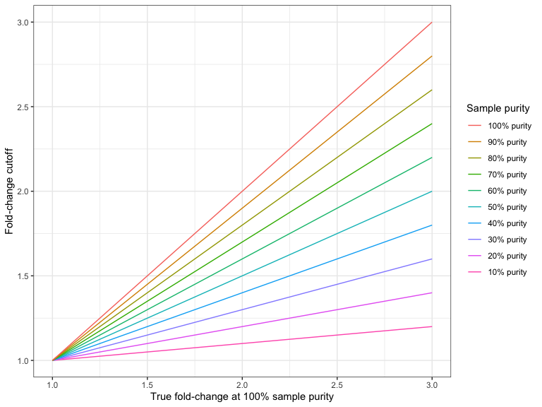
Figure 24.7: The required fold-change cutoff to detect amplifications of different magnitudes as a function of sample purity.
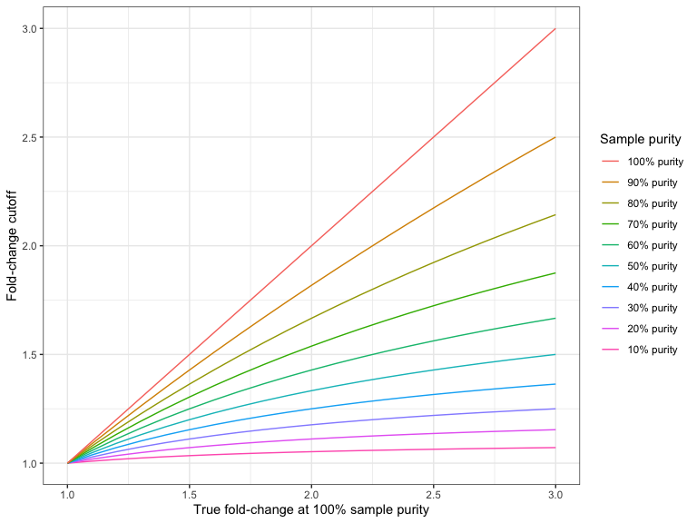
Figure 24.8: The required fold-change cutoff to detect deletions of different magnitudes as a function of sample purity.
The CNV and LOH Detection tool calls CNVs that are both global outliers on the target-level, and locally consistent on the region-level. The tool produces several outputs, which are described below.
Subsections
- Region-level CNV track (Region CNVs)
- Target-level CNV track (Target CNVs)
- Gene-level annotation track (Gene CNVs)
- Loss-of-heterozygosity track
- CNV results report
- CNV algorithm report