- Preliminary steps to run the Type Among Multiple Species workflow
- How to run the Type Among Multiple Species workflow
- Example of results obtained using the Type Among Multiple Species workflow
Type Among Multiple Species
The Type Among Multiple Species workflow is designed for typing a sample among multiple predefined species (figure 13.49).
Figure 13.49: Overview of the template Type Among Multiple Species workflow.
It allows identification of the closest matching reference species among the user specified reference list(s) which may represent multiple species. The workflow identifies the associated MLST scheme and type, determines variants found when mapping the sample data against the identified best matching reference, and finds occurring resistance genes if they match genes within the user specified resistance database.
The workflow also automatically associates the analysis results to the user specified Result Metadata Table. For details about searching and quick filtering among the sample metadata and generated analysis result data (see Filtering in Result Metadata Table).
Preliminary steps to run the Type Among Multiple Species workflow
Before starting the workflow,
- Download microbial genomes using either the Download Custom Microbial Reference Database tool, the prokaryotic databases from the Download Curated Microbial Reference Database tool or the Download Pathogen Reference Database tool (see the Working with databases chapter). Databases can also be created using the Update Sequence Attributes in Lists tool.
- Download the MLST schemes using the Download MLST Scheme tool (see Download MLST Scheme).
- Download the database for the Find Resistance with Nucleotide DB tool using the Download Resistance Database tool (see the Download Resistance Database section).
- Create a New Result Metadata table using the Create Result Metadata Table tool (see the Create Result Metadata Table section).
When you are ready to start the workflows, your navigation area should look similar to the figure 13.50.
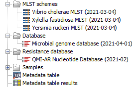
Figure 13.50: Overview of the Navigation area after creating the result metadata table and downloading the databases and MLST schemes necessary to run the workflows.
How to run the Type Among Multiple Species workflow
To run the workflow for one or more samples containing multiple species, go to
Toolbox | Template Workflows (![]() ) | Microbial Workflows (
) | Microbial Workflows (![]() ) | Typing and Epidemiology (
) | Typing and Epidemiology (![]() ) | Type Among Multiple Species (
) | Type Among Multiple Species (![]() )
)
- Specify the sample(s) or folder(s) of samples you would like to type (figure 13.51) and click Next. Remember that if you select several items, they will be run as batch units.
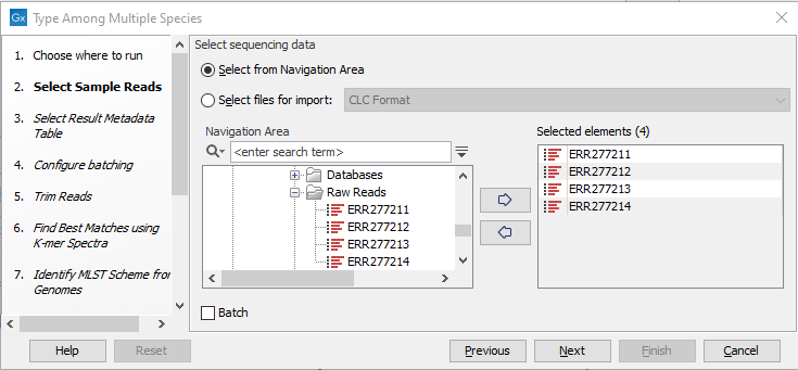
Figure 13.51: Select the reads from the sample(s) you would like to type. - Specify the Result Metadata Table you want to use (figure 13.52) and click Next.
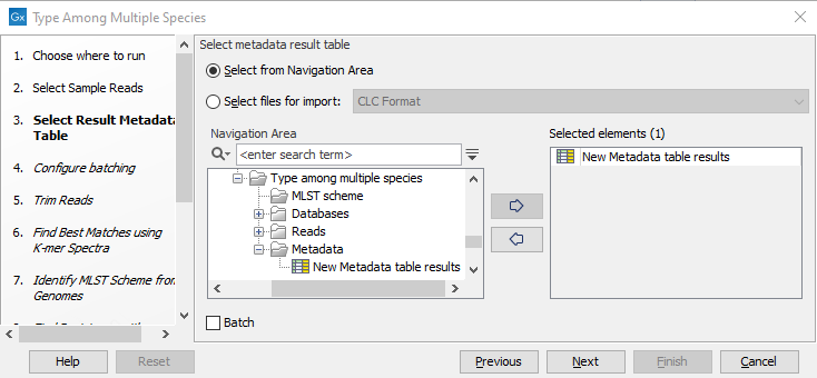
Figure 13.52: Select the metadata table you would like to use. - Define batch units using organisation of input data to create one run per input or use a metadata table to define batch units. Click Next.
- The next wizard window gives you an overview of the samples present in the selected folder(s). Choose which of these samples you want to analyze in case you are not interested in analyzing all the samples from a particular folder (figure 13.53).
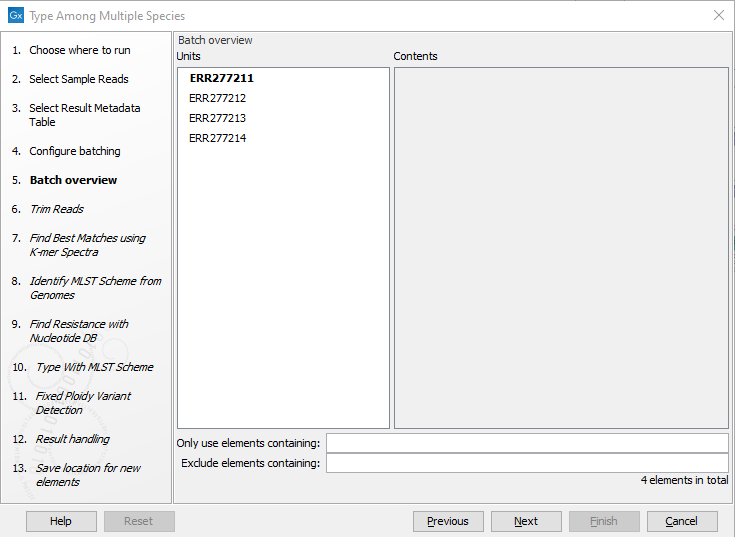
Figure 13.53: Choose which of the samples present in the selected folder(s) you want to analyze. - You can specify a trim adapter list and set up parameters if you would like to trim your sequences from adapters. Specifying a trim adapter list is optional but recommended to ensure the highest quality data for your typing analysis (figure 13.54). Learn about trim adapter lists at http://resources.qiagenbioinformatics.com/manuals/clcgenomicsworkbench/current/index.php?manual=Trim_adapter_list.html.
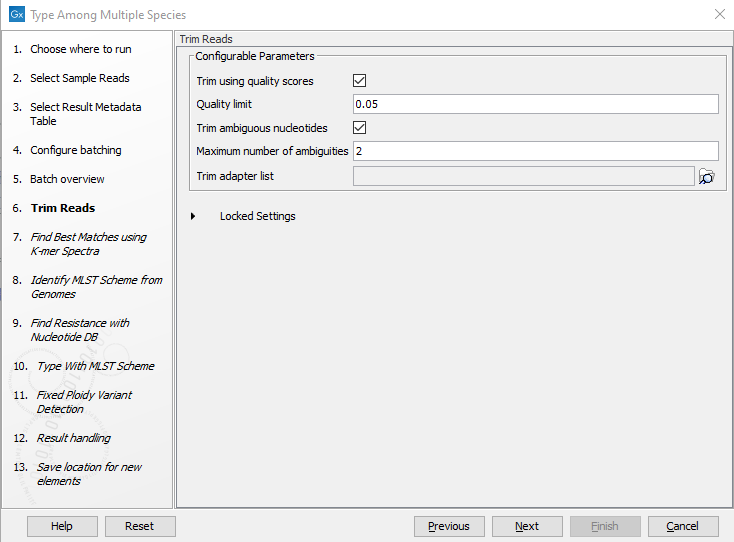
Figure 13.54: You can choose to trim adapter sequences from your sequencing reads.The parameters that can be set are:
- Trim ambiguous nucleotides: if checked, this option trims the sequence ends based on the presence of ambiguous nucleotides (typically N).
- Maximum number of ambiguities: defines the maximal number of ambiguous nucleotides allowed in the sequence after trimming.
- Trim using quality scores: if checked, and if the sequence files contain quality scores from a base-caller algorithm, this information can be used for trimming sequence ends.
- Quality limit: defines the minimal value of the Phred score for which bases will not be trimmed.
- Choose the species-specific references to be used by the Find Best Matches using K-mer Spectra tool (figure 13.55). The list can be a fully customized list, the downloaded bacterial genomes from NCBI list (see section 18.1.1) or a subset of it. Click Next.
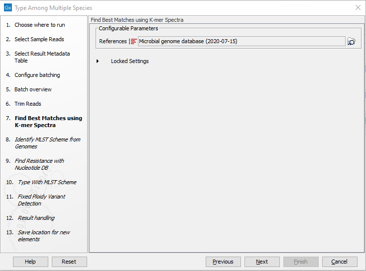
Figure 13.55: Specify the references for the Find Best Matches using K-mer Spectra tool. - Specify MLST schemes to be used for the Identify MLST Scheme from Genomes tool so they correspond to corresponding to the chosen reference list(s) (figure 13.56).
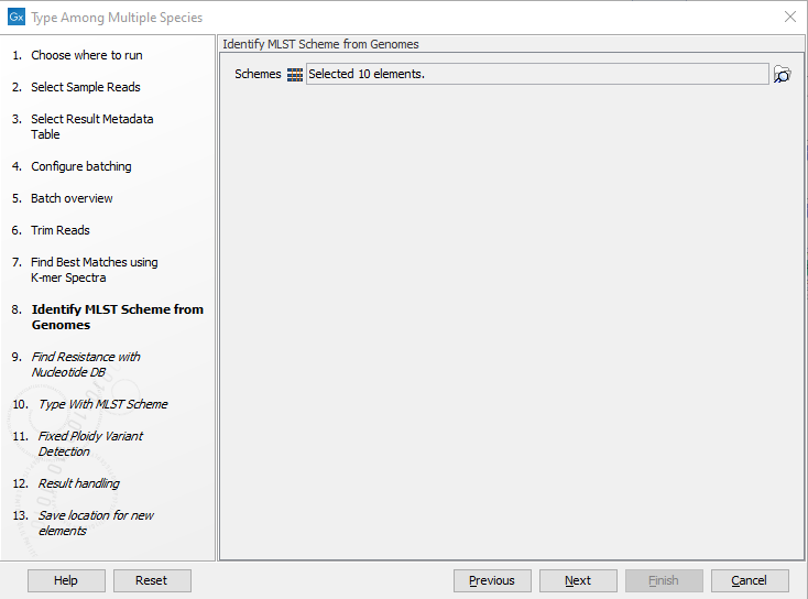
Figure 13.56: Specify the schemes that best describe your sample(s). - Specify the resistance database (figure 13.57) and set the parameters for the Find Resistance with Nucleotide DB tool.
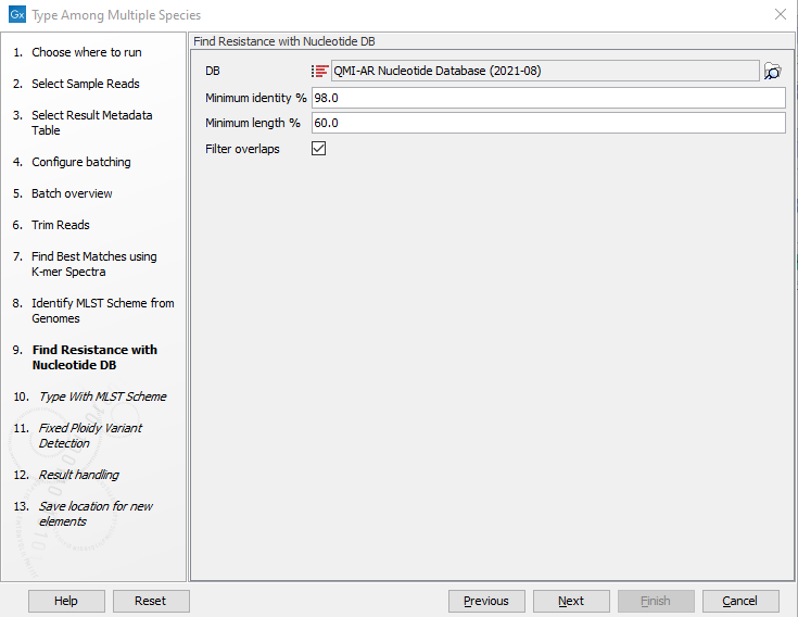
Figure 13.57: Specify the resistance database to be used for the Find Resistance with Nucleotide DB tool.The parameters that can be set are:
- Minimum Identity %: is the threshold for the minimum percentage of nucleotides that are identical between the best matching resistance gene in the database and the corresponding sequence in the genome.
- Minimum Length %: reflect the percentage of the total resistance gene length that a sequence must overlap a resistance gene to count as a hit for that gene. Here represented as a percentage of the total resistance gene length.
- Filter overlaps: will perform extra filtering of results per contig, where one hit is contained by the other with a preference for the hit with the higher number of aligned nucleotides (length * identity).
Click Next.
- Specify the parameters for the Type with MLST Scheme tool (figure 13.58).
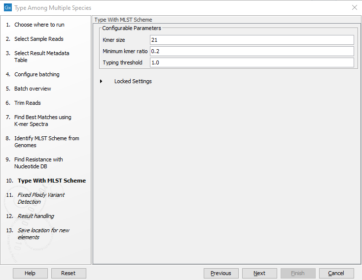
Figure 13.58: Specify the parameters for MLST typing.The parameters that can be set are:
- Kmer size: determines the number of nucleotides in the kmer - raising this setting might increase specificity at the cost of some sensitivity.
- Typing threshold: determines how many of the kmers in a sequence type that needs to be identified before a typing is considered conclusive. The default setting of 1.0 means that all kmers in all alleles must be matched.
- Minimum kmer ratio: the minimum kmer ratio of the least occurring kmer and the average kmer hit count. If an allele scores higher than this threshold it is classified as a high-confidence call.
Click Next.
- Specify the parameters for the Fixed Ploidy Variant Detection tool (figure 13.59) before clicking Next.
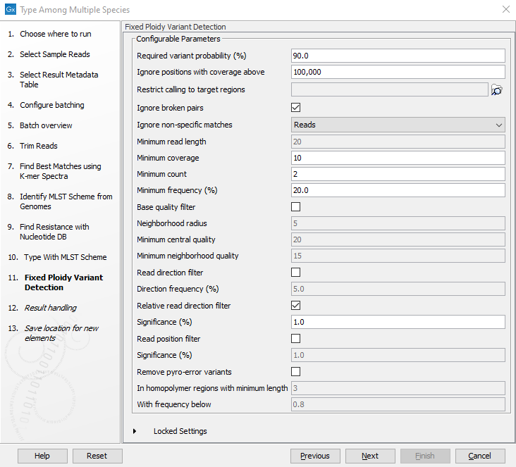
Figure 13.59: Specify the parameters to be used for the Fixed Ploidy Variant Detection tool.The parameters that can be set are:
- Required variant probability (%): The 'Required variant probability' is the minimum probability value of the 'variant site' required for the variant to be called. Note that it is not the minimum value of the probability of the individual variant. For the Fixed Ploidy Variant detector, if a variant site - and not the variant itself - passes the variant probability threshold, then the variant with the highest probability at that site will be reported even if the probability of that particular variant might be less than the threshold. For example if the required variant probability is set to 0.9 then the individual probability of the variant called might be less than 0.9 as long as the probability of the entire variant site is greater than 0.9.
- Ignore positions with coverage above: Ignore positions with a read-coverage larger than this value.
- Restrict calling to target regions: Select a region track to specify the regions in which variants should be called.
- Ignore broken pairs: You can choose to ignore broken pairs by clicking this option.
- Ignore non-specific matches: You can choose to ignore non-specific matches between reads, regions or to not ignore them at all.
- Minimum read length: Only variants in reads longer than this size are called.
- Minimum coverage: Only variants in regions covered by at least this many reads are called.
- Minimum count: Only variants that are present in at least this many reads are called.
- Minimum frequency %: Only variants that are present at least at the specified frequency (calculated as count/coverage) are called.
- Base quality filter: The base quality filter can be used to ignore the reads whose nucleotide at the potential variant position is of dubious quality.
- Neighborhood radius: Determine how far away from the current variant the quality assessment should extend.
- Minimum central quality: Reads whose central base has a quality below the specified value will be ignored. This parameter does not apply to deletions since there is no "central base" in these cases.
- Minimum neighborhood quality: Reads for which the minimum quality of the bases is below the specified value will be ignored.
- Read direction filters: The read direction filter removes variants that are almost exclusively present in either forward or reverse reads.
- Direction frequency %: Variants that are not supported by at least this frequency of reads from each direction are removed.
- Relative read direction filter: The relative read direction filter attempts to do the same thing as the Read direction filter, but does this in a statistical, rather than absolute, sense: it tests whether the distribution among forward and reverse reads of the variant carrying reads is different from that of the total set of reads covering the site. The statistical, rather than absolute, approach makes the filter less stringent.
- Significance %: Variants whose read direction distribution is significantly different from the expected with a test at this level, are removed. The lower you set the significance cut-off, the fewer variants will be filtered out.
- Read position filter: It removes variants that are located differently in the reads carrying it than would be expected given the general location of the reads covering the variant site.
- Significance %: Variants whose read position distribution is significantly different from the expected with a test at this level, are removed. The lower you set the significance cut-off, the fewer variants will be filtered out.
- Remove pyro-error variants: This filter can be used to remove insertions and deletions in the reads that are likely to be due to pyro-like errors in homopolymer regions. There are two parameters that must be specified for this filter:
- In homopolymer regions with minimum length: Only insertion or deletion variants in homopolymer regions of at least this length will be removed.
- With frequency below: Only insertion or deletion variants whose frequency (ignoring all non-reference and non-homopolymer variant reads) is lower than this threshold will be removed.
- In the Result handling window, pressing the button Preview All Parameters allows you to preview - but not change - all parameters. Choose to save the results (we recommend to create a new folder to this effect) and click on the button labeled Finish.
Outputs are generated on a per sample basis and on a summary level. You can find them all in the new folder you created to save them (figure 13.60), but those marked with a (*) have also been added automatically to the New Metadata Result Table (see the section Example of results obtained using the Type a Known Species workflow to understand where your results have been saved).
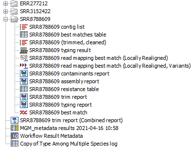
Figure 13.60: Output files from the Type Among Multiple Species workflow.
For each sample, the following outputs are generated:
- Trim report: report from the Trim Sequences tool (see http://resources.qiagenbioinformatics.com/manuals/clcgenomicsworkbench/current/index.php?manual=Trim_output.html).
- (*)Contaminants report: lists the best match as well as possible contaminants along with coverage level distributions for each reference genome listed.
- (*)Best match: sequence that matches best the data according to the Find Best Matches using K-mer Spectra tool.
- Matches table: contains the best matching sequence, a list of all (maximum 100) significantly matching references and a tabular report on the various statistical values applied.
- Read mapping best match: output from the Local Realignment tool, mapping of the reads using the Best Match as reference.
- Trimmed, cleaned sequences: list of the sequences that were successfully trimmed and mapped to the best reference.
- Assembly summary report: see http://resources.qiagenbioinformatics.com/manuals/clcgenomicsworkbench/current/index.php?manual=De_novo_assembly_report.html.
- Contig list: contig list from the De novo assembly tool.
- (*)Contig list resistance table: result table from the Find Resistance with Nucleotide DB tool, reports the found resistance.
- (*)Typing report: output from the Type with MLST Scheme tool, includes information on which MLST scheme was applied, the best matching sequence type (ST) as well as an overview table with sample information and a table summarizing the allele calls.
- Typing result: output from the Type with MLST Scheme tool, includes information on kmer fractions, kmer hit counts and allele count, identified and called.
- Variant Track: output from the Fixed Ploidy Variant Detection tool. Note that it is possible to export multiple variant track files from monoploid data into a single VCF file with the Multi-VCF exporter. This exporter becomes available when installing the CLC Microbial Genomics Module. All variant track files must have the same reference genome for the Multi-VCF export to work.
For each batch analysis run, the following outputs are generated:
- Combined report: combines the information from the trim report and MLST typing report.
- Results metadata table: a table containing summary information for each sample analyzed and a quick way to find the associated files. In addition, an extra column in the Result Metadata Table called "Best match, average coverage" helps the user to decide if a best match is significant, well covered and of good quality. This is especially helpful when a sample has low quality but is not contaminated.
Example of results obtained using the Type Among Multiple Species workflow
The following example includes typing of 2 samples: 1 Salmonella enterica (acc no. ERR277212), and 1 Yersinia ruckeri (acc no SRR3152422). Using the workflow Type Among Multiple Species workflow, analysis results are automatically summarized in the Result Metadata Table as shown in figure 13.61. The analysis results in this example include resistance found for antibiotic inactivation enzyme, name of the best matching reference, applied MLST scheme, detected sequence type and typing status. You could also choose (using options in the Table Setting window) to display additional information such as the 'Best Match, Species' and 'Find Resistance With Nucleotide DB' for example.
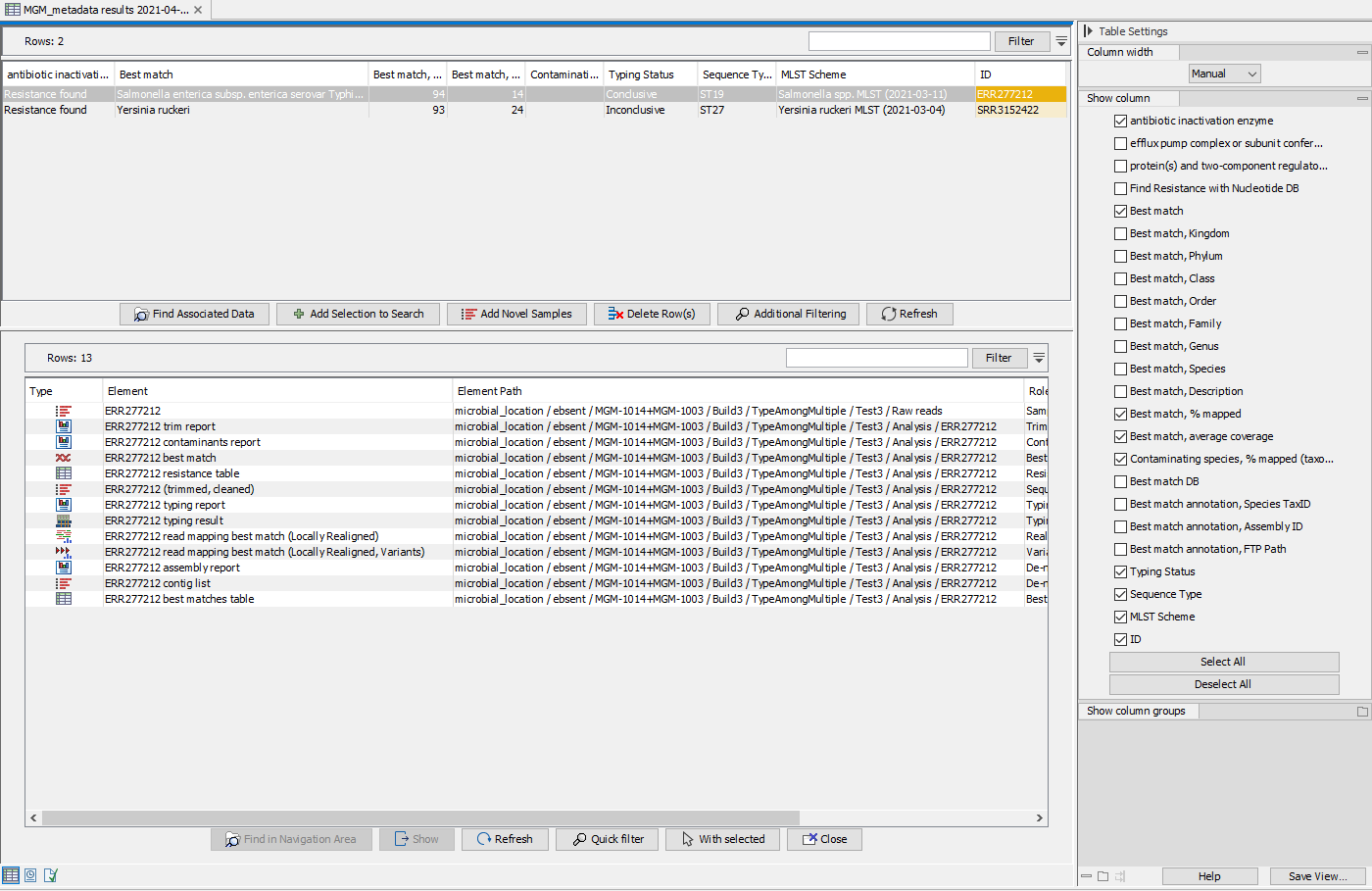
Figure 13.61: View of Result Metadata Table once the Type Among Multiple Species workflow has been executed (top) and associated data elements found (bottom).
Analyzing samples in batch will produce a large amount of output files, making it necessary to filter for the information you are looking for. Through the Result Metadata Table, it is possible to filter among sample metadata and analysis results. By clicking Find Associated Data (![]() ) and optionally performing additional filtering, it is possible to perform additional analyses on a selected subset directly from this Table, such as:
) and optionally performing additional filtering, it is possible to perform additional analyses on a selected subset directly from this Table, such as:
- Generation of SNP trees based on the same reference used for read mapping and variant detection (Create SNP Tree).
- Generation of K-mer Trees for identification of the closest common reference across samples (Create K-mer Tree).
- Run validated workflows (workflows that are associated with a Result Metadata Table and saved in your Navigation Area).
Note that the tool will output, among other files, variant tracks. It is possible to export multiple variant track files from monoploid data into a single VCF file with the Multi-VCF exporter.This exporter becomes available when installing the CLC Microbial Genomics Module. All variant track files must have the same reference genome for the Multi-VCF export to work.