Identify and Annotate Variants (WES)
The Identify and Annotate Variants (WES) ready-to-use workflow should be used to identify and annotate variants in one sample. The workflow is a combination of the Identify Variants and the Annotate Variants workflows.
The workflow starts with mapping the sequencing reads to the human reference sequence, followed by a local realignment to improve the variant detection that is run afterwards. After the variants have been detected, they are annotated with gene names, amino acid changes, conservation scores, information from relevant variants present in the ClinVar database, and information from common variants present in the common dbSNP Common, HapMap, and 1000 Genomes database. Furthermore, a detailed targeted region coverage report is created to inspect the overall coverage and mapping specificity.
Before starting the workflow, you will need to import in the workbench a file with the genomic regions targeted by the amplicon or hybridization kit. Such a file (a BED or GFF file) is usually available from the vendor of the enrichment kit and sequencing machine. Use the Import | Tracks tool to import it in your Navigation Area.
Run the Identify and Annotate Variants (WES) workflow
To run the Identify and Annotate Variants (WES) workflow, go to:
Toolbox | Ready-to-Use Workflows | Whole Exome Sequencing (![]() ) | Somatic Cancer (
) | Somatic Cancer (![]() ) | Identify and Annotate Variants (WES) (
) | Identify and Annotate Variants (WES) (![]() )
)
- Double-click on the workflow name to start the analysis. If you are connected to a server, you will first be asked where you would like to run the analysis.
- First select the sequencing reads from the sample that should be analyzed (figure 14.35).
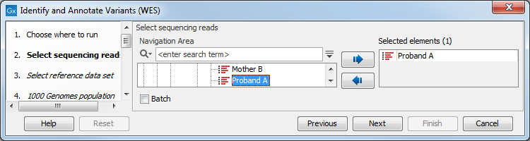
Figure 14.35: Select all sequencing reads from the sample to be analyzed.If several samples should be analyzed, the tool has to be run in batch mode. This is done by checking "Batch" and selecting the folder that holds the data you wish to analyze.
- In the next dialog, you have to select which data set should be used to identify and annotate variants (figure 14.36).
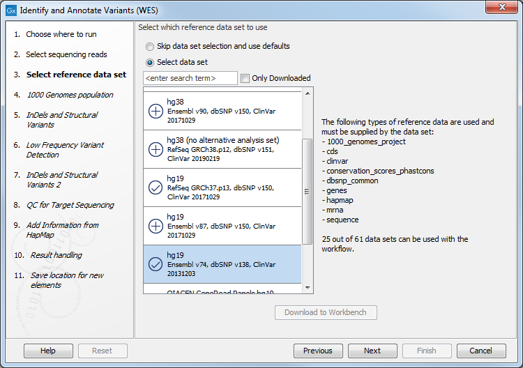
Figure 14.36: Choose the relevant reference Data Set to identify and annotate. - In the next wizard step (figure 14.37) you can select the population from the 1000 Genomes project that you would like to use for annotation.
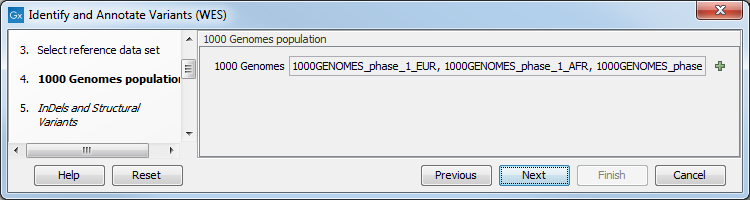
Figure 14.37: Select the population from the 1000 Genomes project that you would like to use for annotation. - In the Indels and Structural Variants dialog (figure 14.38), you
can specify the target regions track. The variants found outside the targeted region will be removed at this step in the workflow, and the output of this step twill be used as guidance in the local realignment.
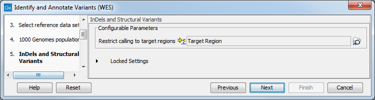
Figure 14.38: In this wizard step you can specify the target regions track. Variants found outside these regions will be removed. - In the next dialog (figure 14.39), you have to specify the parameters for the variant detection. You can again specify the target region track from the earlier step.
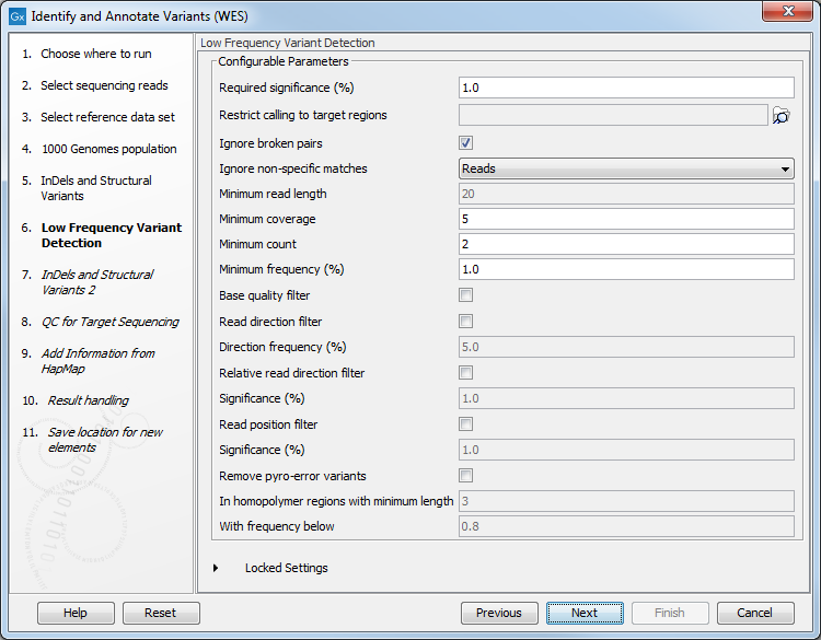
Figure 14.39: Specify the parameters for variant calling.For a description of the different parameters that can be adjusted, see http://resources.qiagenbioinformatics.com/manuals/clcgenomicsworkbench/current/index.php?manual=Low_Frequency_Variant_Detection.html. If you click on "Locked Settings", you will be able to see all parameters used for variant detection in the ready-to-use workflow.
- In the Indels and Structural Variants 2 dialog, you can specify the same target regions track as you did earlier. This step is used to capture Indels and SNVs left after the local realignment has been performed.
- In the QC for Target Sequencing step (figure 14.40) you can select the target region track and specify the minimum read coverage that should be present in the targeted regions.
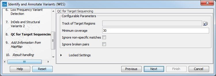
Figure 14.40: Select the track with targeted regions from your experiment. - Finally, select a population from the HapMap database (figure 14.41). This will add information from the Hapmap database to your variants.
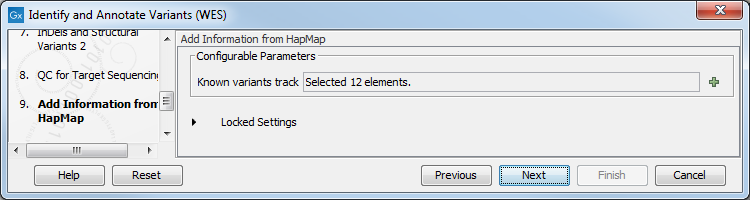
Figure 14.41: Select a population from the HapMap database to add information from the Hapmap database to your variants. - In the last wizard step you can check the selected settings by clicking on the button labeled Preview All Parameters.
In the Preview All Parameters wizard you can only check the settings, and if you wish to make changes you have to use the Previous button from the wizard to edit parameters in the relevant windows.
- Choose to Save your results and click Finish.
Output from the Identify and Annotate Variants (WES) workflow
The Identify and Annotate Variants (WES) workflow produces several outputs.
- Read Mapping (
 ) The mapped sequencing reads. The reads are shown in different colors depending on their orientation, whether they are single reads or paired reads, and whether they map unambiguously (see http://resources.qiagenbioinformatics.com/manuals/clcgenomicsworkbench/current/index.php?manual=Coloring_mapped_reads.html).
- Target Regions Coverage (
 ) The target regions coverage track shows the coverage of the targeted regions. Detailed information about coverage and read count can be found in the table format, which can be opened by pressing the table icon found in the lower left corner of the View Area.
- Target Regions Coverage Report (
 ) The report consists of a number of tables and graphs that in different ways provide information about the targeted regions.
- Structural Variants () Variant track showing the structural variants; insertions, deletions, replacements. Hold the mouse over one of the variants or right-clicking on the variant. A tooltip will appear with detailed information about the variant. The structural variants can also be viewed in table format by switching to the table view. This is done by pressing the table icon found in the lower left corner of the View Area.
- Unfiltered and Filtered Variants (
 ) Variant tracks holding the identified variants before the filters are applied (Unfiltered), and after. Filtered variants are included into 2 separate tracks, one for all identified variants, and one containing larger indels. The variants can be shown in track format or in table format. When holding the mouse over the detected variants in the Track List, a tooltip appears with information about the individual variants. You will have to zoom in on the variants to be able to see the detailed tooltip.
- Amino acid changes Adds information about amino acid changes caused by the variants.
- Track List (
 ) A collection of tracks presented together. Shows the annotated variants track together with the human reference sequence, genes, transcripts, coding regions, the mapped reads, the identified variants, and the structural variants (see figure 14.5).
Please do not delete any of the produced files alone as some of them are linked to other outputs. Please always delete all of them at the same time.
A good place to start is to take a look at the mapping report to see whether the coverage is sufficient in the regions of interest (e.g. > 30 ). Furthermore, please check that at least 90% of the reads are mapped to the human reference sequence. In case of a targeted experiment, please also check that the majority of the reads are mapping to the targeted region.
Next, open the Track List file (see figure 14.42).
The Track List includes a track of the identified annotated variants in context to the human reference sequence, genes, transcripts, coding regions, targeted regions, mapped sequencing reads, relevant variants in the ClinVar database as well as common variants in common dbSNP Common, HapMap, and 1000 Genomes databases.
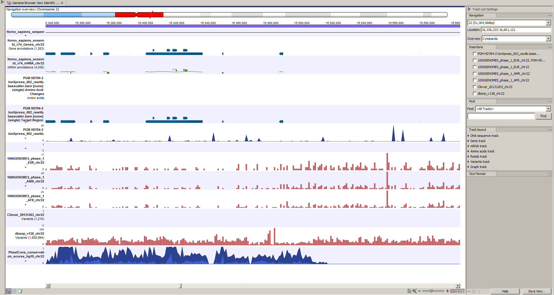
Figure 14.42: Track List to inspect identified variants in the context of the human genome and external databases.
To see the level of nucleotide conservation (from a multiple alignment with many vertebrates) in the region around each variant, a track with conservation scores is added as well.
By double-clicking on the annotated variant track in the Track List, a table will be shown that includes all variants and the added information/annotations (see figure 14.43).
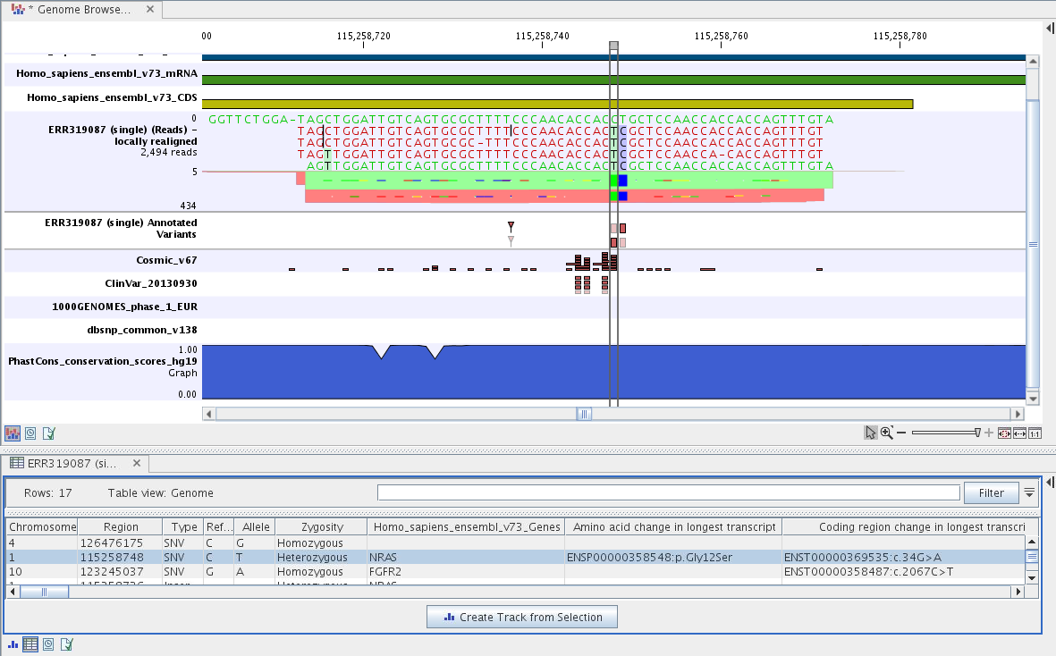
Figure 14.43: Track List with an open track table to
inspect identified somatic variants more closely in
the context of the human genome and external databases.
The added information will help you to identify candidate variants for further research. For example can common genetic variants (present in the HapMap database) or variants known to play a role in drug response or other relevant phenotypes (present in the ClinVar database) easily be seen.
Not identified variants in ClinVar, can for example be prioritized based on amino acid changes (do they cause any changes on the amino acid level?). A high conservation level on the position of the variant between many vertebrates or mammals can also be a hint that this region could have an important functional role and variants with a conservation score of more than 0.9 (PhastCons score) should be prioritized higher. A further filtering of the variants based on their annotations can be facilitated using the table filter on top of the table.
If you wish to always apply the same filter criteria, the Create new Filter Criteria tool should be used to specify this filter and the Identify and Annotate Variants (WES) workflow should be extended by the Identify Candidate Tool (configured with the Filter Criterion). See the reference manual for more information on how preinstalled workflows can be edited.
Please note that in case none of the variants are present in ClinVar or dbSNP Common, the corresponding annotation column headers are missing from the result.
In case you like to change the databases as well as the used database version, please use the Reference Data Manager.