Output from the Identify and Annotate Variants (WES) workflow
The Identify and Annotate Variants (WES) workflow produces several outputs.
- Read Mapping (
 ) The mapped sequencing reads. The reads are shown in different colors depending on their orientation, whether they are single reads or paired reads, and whether they map unambiguously (see http://resources.qiagenbioinformatics.com/manuals/clcgenomicsworkbench/current/index.php?manual=Coloring_mapped_reads.html).
- Target Regions Coverage (
 ) The target regions coverage track shows the coverage of the targeted regions. Detailed information about coverage and read count can be found in the table format, which can be opened by pressing the table icon found in the lower left corner of the View Area.
- Target Regions Coverage Report (
 ) The report consists of a number of tables and graphs that in different ways provide information about the targeted regions.
- Three variant tracks (
 ): Two from the Variant Caller: the Unfiltered Variants is output before the filtering steps, the Variants passing filters is the one used in the Genome Browser View (see
.
http://resources.qiagenbioinformatics.com/manuals/clcgenomicsworkbench/current/index.php?manual=_annotated_variant_table.html for a definition of the variant table content). The third is the Indels indirect evidence track produced by the Structural Variant Caller. This is also available in the Genome Browser View. The variants can be shown in track format or in table format. When holding the mouse over the detected variants in the Track List, a tooltip appears with information about the individual variants. You will have to zoom in on the variants to be able to see the detailed tooltip.
): Two from the Variant Caller: the Unfiltered Variants is output before the filtering steps, the Variants passing filters is the one used in the Genome Browser View (see
.
http://resources.qiagenbioinformatics.com/manuals/clcgenomicsworkbench/current/index.php?manual=_annotated_variant_table.html for a definition of the variant table content). The third is the Indels indirect evidence track produced by the Structural Variant Caller. This is also available in the Genome Browser View. The variants can be shown in track format or in table format. When holding the mouse over the detected variants in the Track List, a tooltip appears with information about the individual variants. You will have to zoom in on the variants to be able to see the detailed tooltip.
- Amino acid changes Adds information about amino acid changes caused by the variants.
- Genome Browser View (
 ) A collection of tracks presented together. Shows the annotated variant track together with the human reference sequence, genes, transcripts, coding regions, amino acid changes, the mapped reads, the identified variants, and the indels indirect evidence variants (see figure 19.5).
Please do not delete any of the produced files alone as some of them are linked to other outputs. Please always delete all of them at the same time.
A good place to start is to take a look at the mapping report to see whether the coverage is sufficient in the regions of interest (e.g. > 30 ). Furthermore, please check that at least 90% of the reads are mapped to the human reference sequence. In case of a targeted experiment, please also check that the majority of the reads are mapping to the targeted region.
Next, open the Genome Browser View (see figure 19.45).
The Genome Browser View includes a track of the identified annotated variants in context to the human reference sequence, genes, transcripts, coding regions, targeted regions, mapped sequencing reads, relevant variants in the ClinVar database as well as common variants in common dbSNP Common, HapMap, and 1000 Genomes databases.
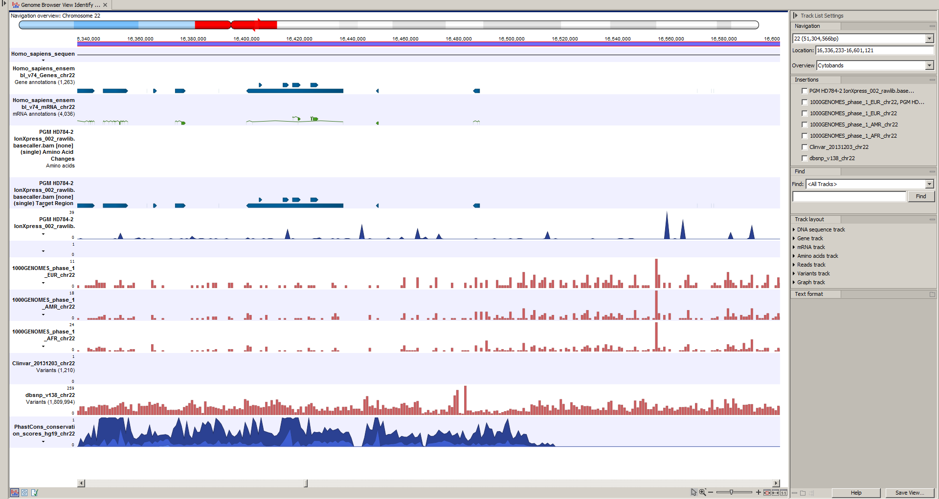
Figure 19.45: Genome Browser View to inspect identified variants in the context of the human genome and external databases.
To see the level of nucleotide conservation (from a multiple alignment with many vertebrates) in the region around each variant, a track with conservation scores is added as well.
By double-clicking on the annotated variant track in the Genome Browser View, a table will be shown that includes all variants and the added information/annotations (see figure 19.46).
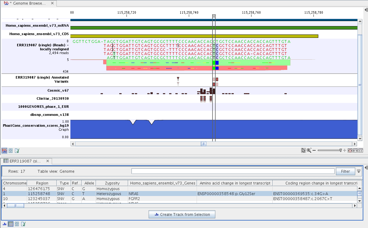
Figure 19.46: Genome Browser View with an open track table to
inspect identified somatic variants more closely in
the context of the human genome and external databases.
The added information will help you to identify candidate variants for further research. For example can common genetic variants (present in the HapMap database) or variants known to play a role in drug response or other relevant phenotypes (present in the ClinVar database) easily be seen.
Not identified variants in ClinVar, can for example be prioritized based on amino acid changes (do they cause any changes on the amino acid level?). A high conservation level on the position of the variant between many vertebrates or mammals can also be a hint that this region could have an important functional role and variants with a conservation score of more than 0.9 (PhastCons score) should be prioritized higher. A further filtering of the variants based on their annotations can be facilitated using the table filter on top of the table.
If you wish to always apply the same filter criteria, the Create new Filter Criteria tool should be used to specify this filter and the Identify and Annotate Variants (WES) workflow should be extended by the Identify Candidate Tool (configured with the Filter Criterion). See the reference manual for more information on how preinstalled workflows can be edited.
Please note that in case none of the variants are present in ClinVar or dbSNP Common, the corresponding annotation column headers are missing from the result.
In case you like to change the databases as well as the used database version, please use the Reference Data Manager.