Alpha Diversity
Alpha diversity is the diversity within a particular area or ecosystem, usually expressed by the number of species (i.e., species richness) in that ecosystem. Alpha diversity estimates are calculated from a series of rarefaction analyses and hence dependent on sampling depth.
The Alpha diversity tool takes abundance tables as input. Abundance tables can be generated in the workbench by the following three tools: OTU clustering, Build Functional Profile and Taxonomic Profiling. With the first two tools, the abundance tables generated are count-based, and Alpha diversity measures calculated from such tables give an absolute number of species. However, when using an abundance table generated by the Taxonomic Profiling tool, Alpha diversity results will not give an absolute number of species, but rather estimates that are useful for comparative studies, i.e., to assess the depth of sequencing, or to compare different communities.
To run the tool. go to:
Metagenomics (![]() ) | Abundance Analysis (
) | Abundance Analysis (![]() ) | Alpha Diversity (
) | Alpha Diversity (![]() )
)
Choose an abundance table to use as input.
The next wizard window offers you to set up different analysis parameters (figure 7.1).
For example, you can calculate metrics at a specific taxonomic level: the tool will then aggregate the features by taxonomy (so that OTUs from the same phylum will be grouped together) before computing the metric. The default value is to not aggregate by taxonomy. You then select which diversity measures to calculate (see Alpha diversity measures).
If you are working with OTU abundance tables, you can also specify an appropriate phylogenetic tree for computing phylogenetic diversity. In that case, you must have aligned the OTUs and constructed a phylogeny before running the Alpha Diversity tool. Note that the "Evaluate at taxonomic level" option described above does not apply to the "Phylogenetic Diversity" metric, since that metric is not using taxonomic information, but is making use of a phylogenetic tree based on OTU sequences.
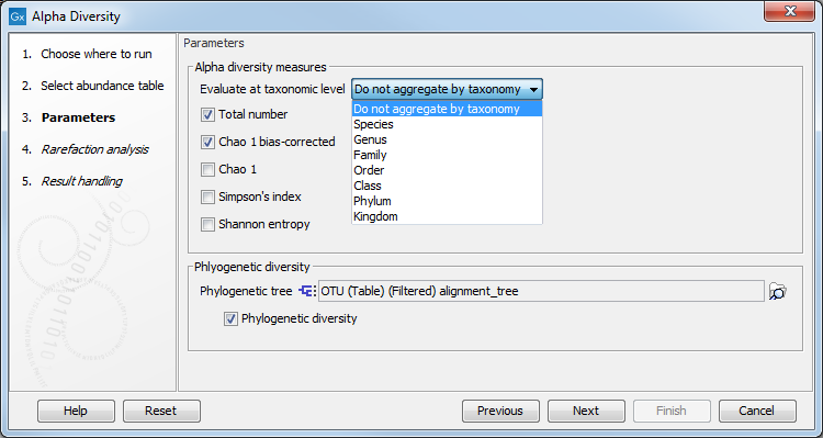
Figure 7.1:
Set up parameters for the Alpha Diversity tool.
In the following dialog (figure 7.2), set up the rarefaction analysis parameters.
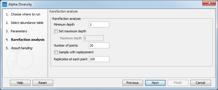
Figure 7.2:
Set up parameters for the Rarefaction analysis.
The rarefaction analyses are done differently depending on the type of abundance table used as input. For OTU and functional abundance tables, where abundances are counts, rarefaction is calculated by sub-sampling the abundances in the different samples at different depths. For whole metagenome taxonomic profiling abundance tables, where abundances are coverage estimates, sub-sampling is not possible, so diversity is estimated using a probabilistic model corresponding to our qualification criteria instead (see Taxonomic Profiling).
The rarefaction analysis parameters will define the granularity of the alpha diversity curve.
- Minimum depth to sample is set to 1 by default.
- Maximum depth to sample If this option is not checked, the maximum depth is set it to the total number of reads (in the case of one sample) or the total number of reads of the sample with most reads.
- Numbers of points Number of different depths to be sampled. For example, if you choose to sample 5 depths between 1000 and 5000, the algorithm will sub-sample each sample at 1000, 2000, 3000, 4000, and 5000 reads.
- Sample with replacement Whether the sampling should be performed with or without replacement.
- Replicates at each depth (for counts-based abundance tables only). How many times the algorithm sub-samples the data at each depth.
The tool will generate a graph for each selected Alpha diversity measure (figure 7.3). Using the Lines and dots editor on the right hand side panel, it is possible to color samples according to groups defined by associated metadata. Note that you can filter metadata by typing the appropriate text in the field above each list of metadata elements. This is an easy way to change the visualization of a group of data at once.
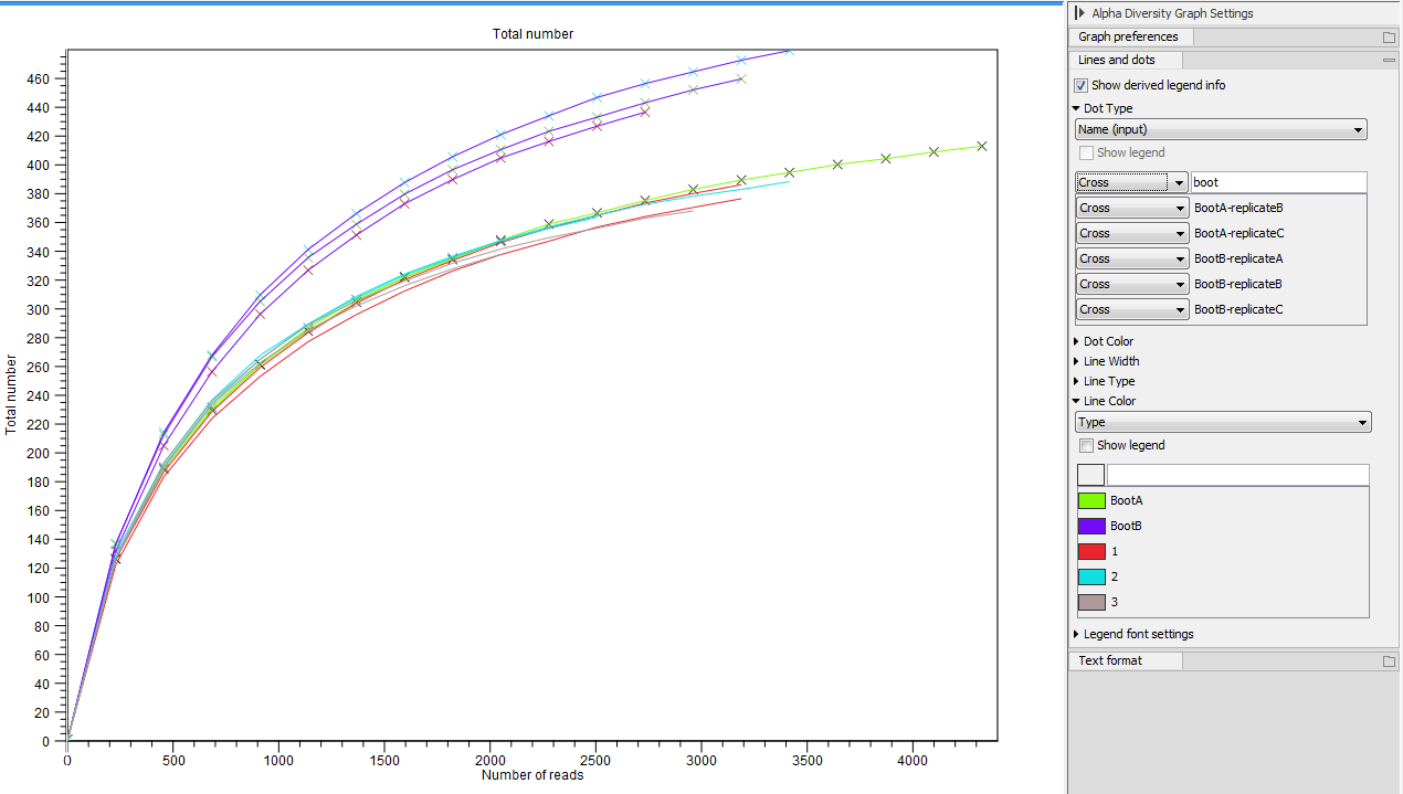
Figure 7.3:
An example of Alpha Diversity graph based on phylogenetic diversity.
Note that the option "Show derived legend info" is enabled by default (figure 7.4). According to this setting, the legend(s) for which metadata categories happen to be "shared" for all items in the legend will display the dependencies between the different categories. In this example, the "Location" category determines Dot Type, and the "Antibiotic" category determines Line Color. For this particular data set, all samples with a specific location have the same antibiotic resistance. The "Show derived legend info" option enables the legends to show such implicit dependencies in the data. If such a visualization is not wished for, the option can be disabled, and the legend will show only the metadata category values that were explicitly selected in the right hand side panel.
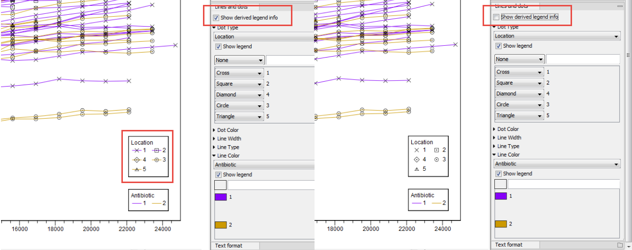
Figure 7.4:
Example of the difference between having the "Show derived legend info" enabled or disabled. When enabled, the legend helps visualize that "location" and "antibiotic" are dependent for this particular data set.
It is also possible to view the Alpha diversity measures as Box plot to see if samples of a certain group are significantly different than those of other groups (figure 7.5). For example, one can check if soils of a certain type contain more bacterial species than other samples.
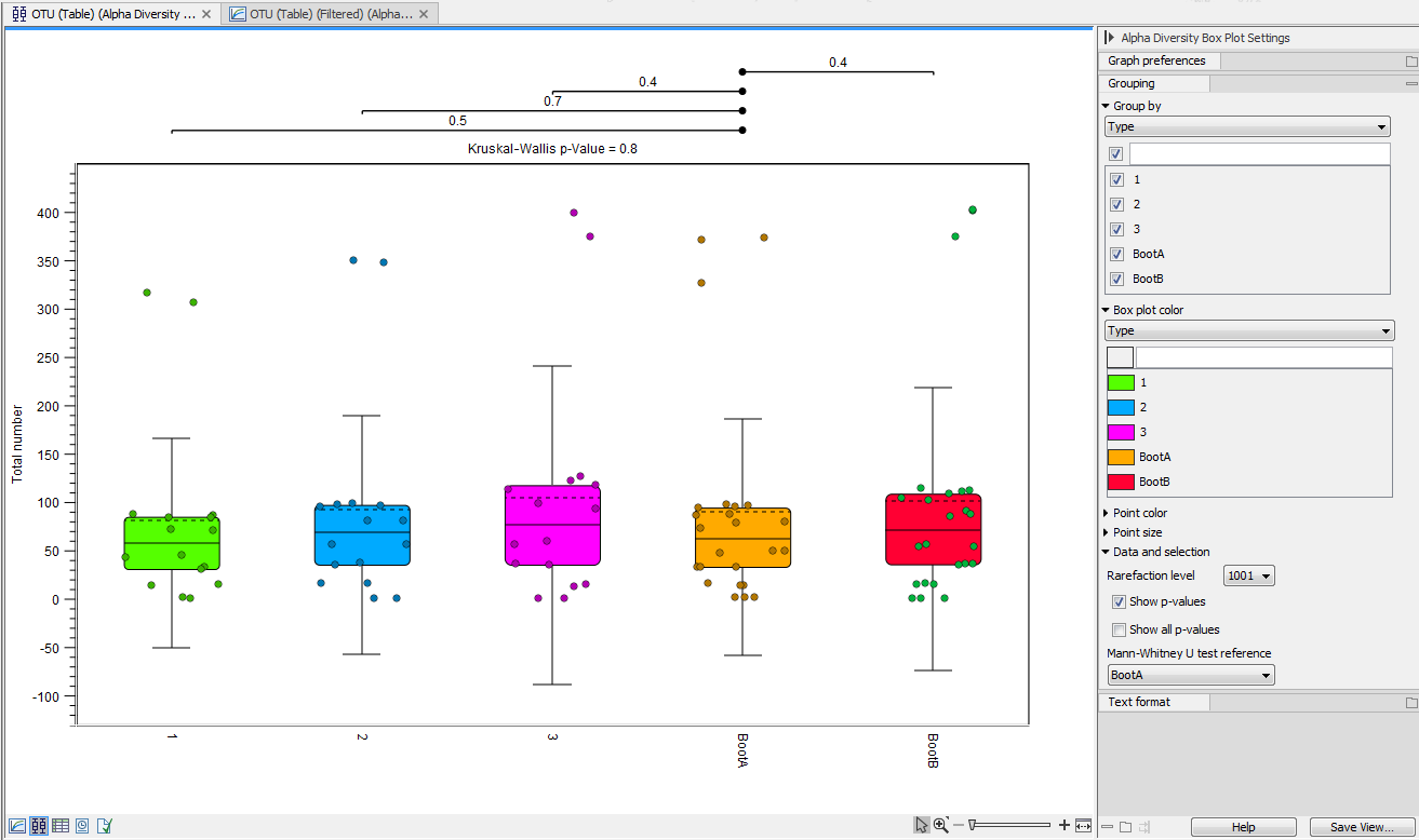
Figure 7.5:
Alpha diversities shown in a box plot.
The box plot view can also display the following statistics:
- Rarefaction level This drop down menu allows to choose which value of the rarefaction curve should be used. The values of "Rarefaction level" are the same as the horizontal axis in the Alpha Diversity Graph view and correspond to the depths at which the input data is sub-sampled before calculating the diversity metric in the Alpha Diversity tool.
- Kruskal-Wallis H test This test is used to assess whether the values originate from the same distribution or whether their distribution is different depending on the group they belong to. This test is a nonparametric alternative to ANOVA (i.e., it does not depend on the data following a given distribution - the normal distribution in case of ANOVA). A significant p-value for the Kruskal-Wallis test means that at least one group follows a different distribution, but does not specify which pairs have different distributions.
- Mann-Whitney U test The tool therefore performs a pair-wise Mann-Whitney U test to specifically determine which pairs of groups follow different distributions.
These statistical tests are performed when the "Show p-values" option is checked. If the "Show all p-values" is checked, all pairwise Mann-Whitney U tests are performed, while when it is not checked, only the pairs that contain the reference group specified in the "Mann-Whitney U test reference" option are considered.
Subsections