Beta Diversity
Beta diversity examines the change in species diversity between ecosystems.
The analysis is done in two steps. First, the tool estimates a distance between each pair of samples (see Beta diversity measures). Once the distance matrix is calculated, the beta diversity analysis tool performs Principal Coordinate Analysis (PCoA) on the distance matrices. These can be visualized by selecting the PCoA icon (![]() ) in the bottom of the Beta Diversity results (
) in the bottom of the Beta Diversity results (![]() ).
).
If you are working with an OTU table, you can specify an appropriate phylogenetic tree for computing phylogenetic diversity. In that case, you must have aligned the OTUs and constructed a phylogeny before running the Beta Diversity tool.
To run the tool, open
Metagenomics (![]() ) | Abundance Analysis (
) | Abundance Analysis (![]() ) | Beta Diversity (
) | Beta Diversity (![]() )
)
Select an abundance table with more than one sample as input (i.e., an OTU table table, or a merged functional or profiling table) and set the parameters for the beta diversity analysis as shown in figure 7.6.
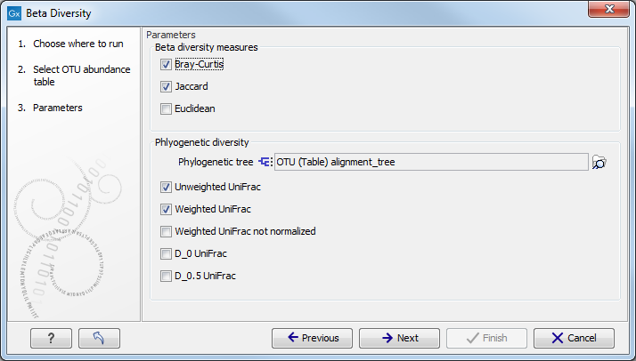
Figure 7.6:
Set up parameters for the Beta diversity tool.
The output of the tool is a 3D PCoA plot (figure 7.7) that can also be seen as a table or a 2D Principal Coordinate Plot.
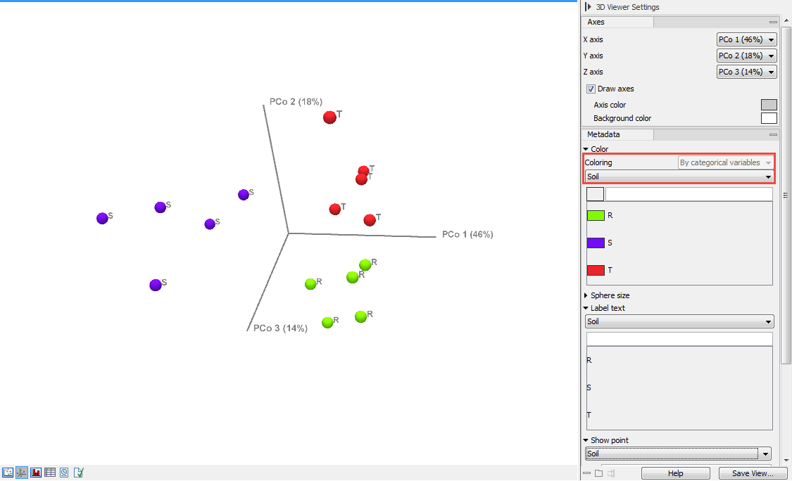
Figure 7.7:
Beta diversity results seen as a 3D PCoA, with coloring done according to the categories dedined by the metadata.
Use the settings in the right hand Side Panel of the PCoA (2D or 3D) to modify the plot visualization.
In the section Metadata, the Color menu (1) allows you to choose whether you want your data to be colored according to categorical variables (the ones defined by the metadata, as seen in figure 7.7) or by abundance values (figure 7.8).
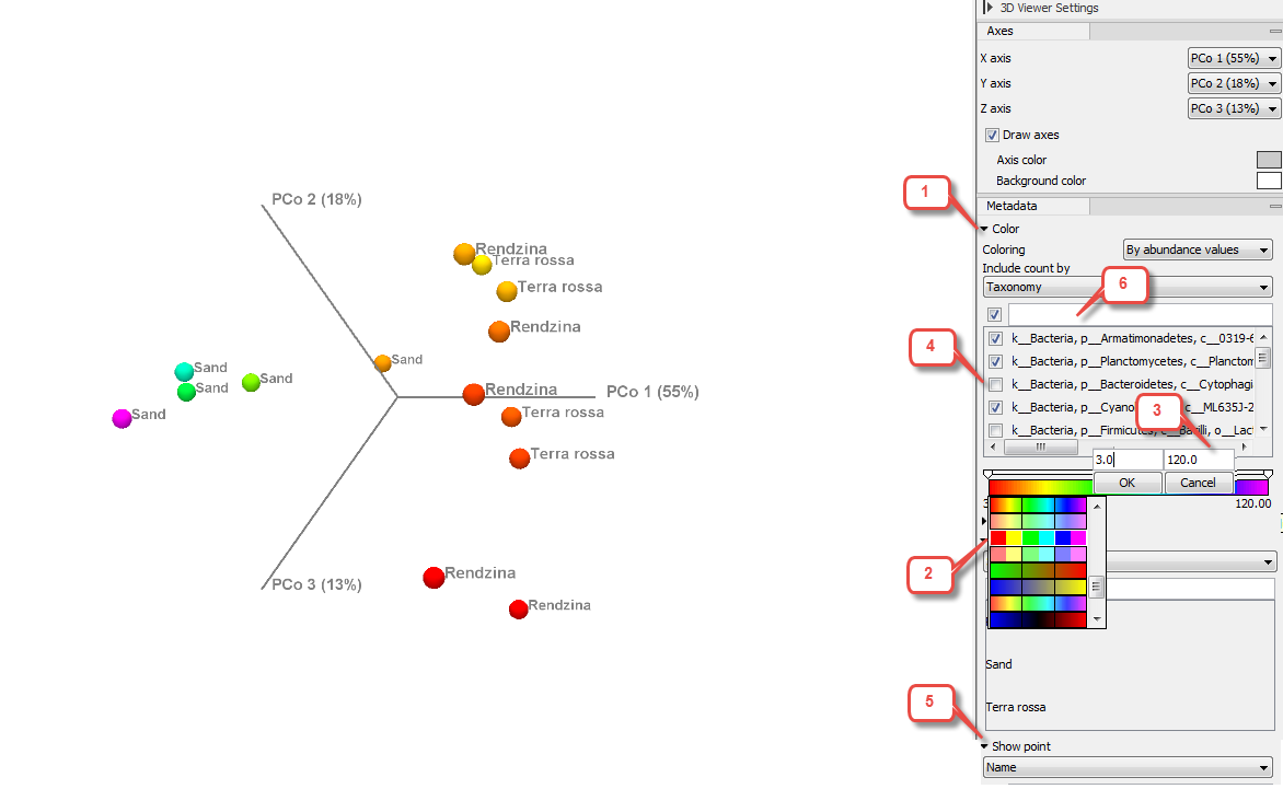
Figure 7.8:
Beta diversity results seen as a 3D PCoA, with coloring done according to taxonomic abundance values.
Coloring per abundance values is done with a gradient scheme. Click on the gradient bar to choose from several color schemes (2). Double-click on the slider to set specific values for the gradient (3).
When coloring "By abundance values", it is possible to control the abundance value calculation through existing metadata fields: Name, Taxonomy or, in the case of OTU abundance tables, Sequence. The drop down menu will then display the items that can be deselected (4) if you want to remove them from the abundance value calculation: this will not remove any of the data point from the PCoA view, but just change the abundance values of the affected point and therefore its coloring. To remove a data point from the plot, use the Show point menu (5) below in the Side Panel.
As in other metadata Side Panel features, use the field above each menu (6) to filter that menu. This is particularly helpful when menus are very long, as is the case with taxonomies for example.
Subsections