Process tagged sequences
Multiplexing based on the name of the sequence is of course only possible if proper sequence names could be assigned from the sequencing process. With many of the new high-throughput technologies, this is not possible.However, there is a need for being able to input several different samples to the same sequencing run, so multiplexing is still relevant - it just has to be based on another way of identifying the sequences. A method has been proposed to tag the sequences with a unique identifier during the preparation of the sample for sequencing [Meyer et al., 2007].
With this technique, each sequence will have a sample-specific tag - a special sequence of nucleotides before and after the sequence of interest. This principle is shown in figure 18.6 (please refer to [Meyer et al., 2007] for more detailed information).
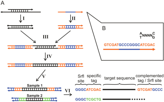
Figure 18.6: Tagging the target sequence. Figure from [Meyer et al., 2007].
The sample-specific tag - also called the barcode - can then be used to distinguish between the different samples when analyzing the sequence data. This post-processing of the sequencing data has been made easy by the multiplexing functionality of the CLC Main Workbench which simply divides the data into separate groups prior to analysis. Note that there is also an example using Illumina data here.
The first step is to separate the imported sequence list into sublists based on the barcode of the sequences:
Toolbox | NGS Core Tools (![]() ) | Multiplexing (
) | Multiplexing (![]() ) | Process Tagged Sequences (
) | Process Tagged Sequences (![]() )
)
This opens a dialog where you can add the sequences you wish to sort. You can also add sequence lists.
When you click Next, you will be able to specify the details of how the de-multiplexing should be performed. At the bottom of the dialog, there are three buttons which are used to Add, Edit and Delete the elements that describe how the barcode is embedded in the sequences.
First, click Add to define the first element. This will bring up the dialog shown in 18.7.
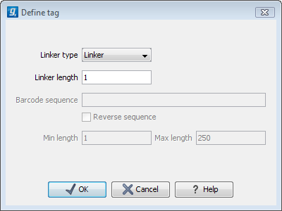
Figure 18.7: Defining an element of the barcode system.
At the top of the dialog, you can choose which kind of element you wish to define:
- Linker. This is a sequence which should just be ignored - it is neither the barcode nor the sequence of interest. Following the example in figure 18.6, it would be the four nucleotides of the SrfI site. For this element, you simply define its length - nothing else.
- Barcode. The barcode is the stretch of nucleotides used to group the sequences. For that, you need to define what the valid bases are. This is done when you click Next. In this dialog, you simply need to specify the length of the barcode.
- Sequence. This element defines the sequence of interest. You can define a length interval for how long you expect this sequence to be. The sequence part is the only part of the read that is retained in the output. Both barcodes and linkers are removed.
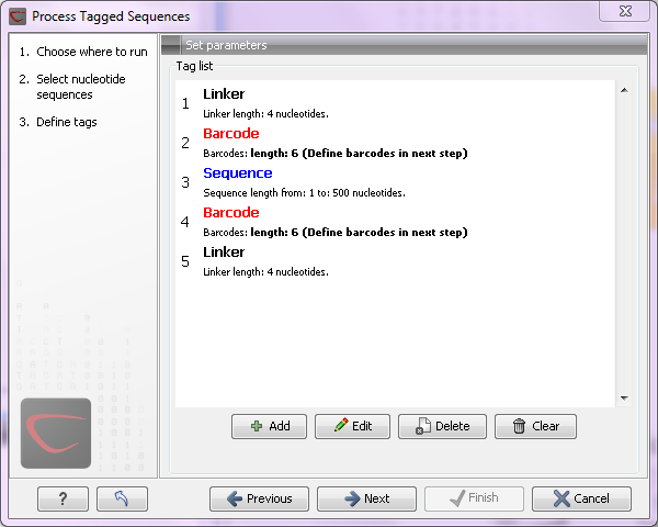
Figure 18.8: Processing the tags as shown in the example of figure 18.6.
If you have paired data, the dialog shown in figure 18.8 will be displayed twice - one for each part of the pair.
Clicking Next will display a dialog as shown in figure 18.9.
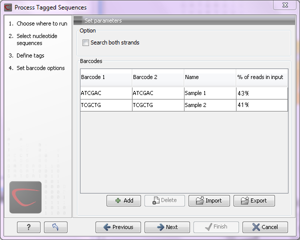
Figure 18.9: Specifying the barcodes as shown in the example of figure 18.6.
The barcodes can be entered manually by clicking the Add (![]() ) button. You can edit the barcodes and the names by clicking the cells in the table. The name is used for naming the results.
) button. You can edit the barcodes and the names by clicking the cells in the table. The name is used for naming the results.
In addition to adding barcodes manually, you can also Import (![]() ) barcode definitions from an Excel or CSV file. The input format consists of two columns: the first contains the barcode sequence, the second contains the name of the barcode. An acceptable csv format file would contain columns of information that looks like:
) barcode definitions from an Excel or CSV file. The input format consists of two columns: the first contains the barcode sequence, the second contains the name of the barcode. An acceptable csv format file would contain columns of information that looks like:
| "AAAAAA","Sample1" |
| "GGGGGG","Sample2" |
| "CCCCCC","Sample3" |
The Preview column will show a preview of the results by running through the first 10,000 reads.
At the top, you can choose to search on both strands for the barcodes (this is needed for some 454 protocols where the MID is located at either end of the read).
Click Next to specify the output options. First, you can choose to create a list of the reads that could not be grouped. Second, you can create a summary report showing how many reads were found for each barcode (see figure 18.10).
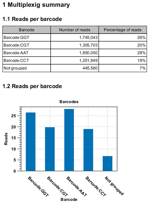
Figure 18.10: An example of a report showing the number of reads in each group.
There is also an option to create subfolders for each sequence list. This can be handy when the results need to be processed in batch mode.
A new sequence list will be generated for each barcode containing all the sequences where this barcode is identified. Both the linker and barcode sequences are removed from each of the sequences in the list, so that only the target sequence remains. This means that you can continue the analysis by doing trimming or mapping. Note that you have to perform separate mappings for each sequence list.
Subsections